Scope of this Book
This book is written with the purpose of establishing the notion that there exists a computationally instantaneous method of arriving at structures of molecules and solids atom-by-atom from first principles without requiring much more than linear equations. This new method is based on the use of transferable atomic sizes obtained using a new paradigm which relies on finding an universal aspect of interactions with electron-positron pairs pre-existing as virtual photons in vacuum polarizations. It gives real-space chemical insights into molecular structure without being constrained in principle by loss of accuracy for large systems. It does not require energy- or density-functionals of wave-function or density-function methods and is therefore computationally very inexpensive.
This book is in two parts. The first part lays down the conceptual and theoretical basis of our quasi-classical approach, which we term as an ab traditio (traditio in Latin means ‘the act of handing over’) approach in which we exploit the feature that the chemical system that is examined is already in its preformed state of rest. This state is described by the m = 0 condition for the chemical potential. Interactions with electron-positron pairs of virtual photons, define atomic sizes at m = 0. They also characterize bond-forming interactions between oppositely and singly charged atomic pairs. This approach is many significant ways different from those invoked since 1925-26 by Schrödinger-Dirac or Heitler-London-Hund-Mulliken theoretical schemes.
The second part of this book is aimed at quantitatively applying our concepts to real systems and to show consistencies with the way of various structures may be interpreted and understood. We succeed in quantitatively accounting for conventional chemical parameters, such as bond-distances, bond angles, coordination numbers, radius ratios, crystal structure, and so on. Our approach is especially applicable to complex biological systems involving molecular docking, clathrate compounds, protein structure, anisotropic crystal systems
Part I: Concepts
In traditional methods of arriving at an ab initio theoretical evaluation of a molecular structure, one starts with isolated atoms of a system and then work out the exponentially walled, time-consuming way they interact in phase space to arrive at an energy-optimized or density-optimized stationary or ground state of interest. Such stationary states are¾in the definition of Bohr229¾“states of the system in which there is no radiation of energy, states which consequently will be stationary as long as the system is not disturbed from outside.” Such a state does not radiate or absorb energy in the absence of an external perturbation or change in potential. The chemist’s primary interest in molecular structure comes therefore mainly after the molecule/crystal has formed and therefore pre-exists in its universal stationary state. The understanding of spatial aspects of every perturbation becomes crucial in understanding responses of molecules to environmental cues. Our approach will be to show that every atom has a core size (which we may call a size eigenfunction) and that every spatial operation leads to a interaction-specific size (a size eigenvalue) to first order.
Instead of understanding from an ab initio perspective (sometimes seemingly stretched to a “creatio ex nihilo” sense) one could as well start a theoretical examination from a pre-existing universal state in an sense. Perhaps the most important ingredient in our approach is the way we look at the chemical potential, m. The usual understanding is that the free-atom m = 0 condition precludes the formation of molecules since atoms react only in the m ¹ 0 condition. Our simplifying contention, on the contrary, is that all the interactions leading to molecule formation requires a m ¹ 0 condition and once the molecule is formed and is in its comfortable stationary state the atom is in a free atom-like condition in the molecule. We find advantage in using a m = 0 condition for the chemical potential for beginning descriptions using traditional first principles of physical chemistry. It is this condition that allows for a first-principles justification of transferable empirical (based on experiments) atomic sizes used so far and that are mainly associated with giants like Bragg, Goldschmidt, Pauling, Shannon. The theoretical justification/understanding of such sizes has been elusive. One of the aims of this book is to provide a simple yet quantitative theoretical insight.
The second important tenet is the existence of vacuum and vacuum polarization as a given. One also needs to assume the electronic configurations of atoms in the periodic table as obtained by spectroscopic methods in the Bohr-Sommerfield era without fundamentally requiring developments of Schrodinger-Dirac or Thomas-Fermi-Kohn methodologies. The starting point and the new paradigm in our exercise is to consider interactions of an atom with a virtual photon involving an electron-positron pair. Given the structure of the atom a positively charged nucleus with negatively charged extra-nuclear electrons balancing the positive charge of the nucleus, we recognize the key feature as the interactions of the extra-nuclear electrons with the positrons of the electron-positron pair. There are direct and indirect interactions of the valence and inner-shell electrons with the positron of the virtual photon. This helps in defining an atom-specific core size, rcore, which has valence-shell and inner-shell contributions.
The quantum aspect that is retained is philosophically and mathematically no more than that used by Feynman for the Bohr model (1913) for hydrogen atom. The Bohr-atom-like feature appears in an inverted sense for the size from valence electrons, when we treat the positron of the virtual photon to be directly in the field of the heavy negative charge of the atom presented by the valence electron. The inner-shell size is dependent on the number of inner-shell electrons which may vary for different conditions of measurement. Having obtained rcore, one then develops atomic sizes, CRP, that is valid for such a state for a given physico-chemical property, P. It is sufficient to use a linear relationship between CRP and rcore.
Examples where inner-shell sizes change considerably when evaluating rcore as compared with those involving chemical equilibrium or stationary states (where m= 0 condition is expected to hold), are those associated with chemical reactivity when m ¹ 0¾such as electronegativity, {rcore}*, or dielectric polarizability, <rcore>. The sizes {rcore}* and <rcore> are related linearly to Pauling’s electronegativity scale, cP, and the atomic dielectric polarizability radius, ra, , respectively. What is so far unforeseen is that the condition for metallic behaviour in elements can be obtained as a simple single-atom criterion {rcore}* ³ aH/2 £ <rcore>, where aH is the Bohr radius of the hydrogen atom.
One sets simple geometrical rules for arriving at the molecular or crystal structure for given bonding situations of interest that can vary within different parts of the same molecule or in different directions for the same atom. Once this is done one arrives at a quantitative real-space model of a molecular structure. In most ab initio methods the most time-consuming step in ab initio molecular structure calculations is in optimizing molecular geometry. This step is now avoided as the molecular structure is obtained directly from inter-atomic distances, the theoretical framework for which is developed by our method. The total energy of this structure can now be quickly calculated, if required, using conventional methods.
In the m = 0 condition of our method, expressions for inter-atomic distances at an equilibrium state will not depend on the strength of a given interaction to first order. The interaction energy is given up (exothermic) or absorbed (endothermic) to reach the m = 0 state. The binding/confining interaction is felt only when the bond is taken out of the m = 0 state. Each time a bond is formed and equilibrium is reached the system is restored to its comfortable m = 0 state until another interaction makes (or breaks) another contact in another direction. Moreover, since we are interested in inter-atomic distances, we are interested only in the 1D component of the interaction in the direction of the interacting atom.
For arriving at the final molecular structure, one requires taking into account the conceptual essentials from many of the other theoretical and experimental results that have evolved since Bohr’s 1913 paper. These include spin statistics, fractional charge, theories of metallization, screening lengths, Fermi-liquid behaviour, superconductivity, emergent phenomena in quantum phase transitions, separation of spin- and charge-times, experiments on electron-positron annihilation, etc. It turns out that one can obtain important quantitative results on molecular/crystal structure once one uses the fundamental concepts behind these advances as given truths.
In our method we find that all bond lengths for a given bond type may be described by a “hub-and-axle” model with atom-specific “hub” sizes and atom-independent “axle” sizes. This “hub-and-axle” nomenclature retains the spirit of the classical mechanical “ball-and-stick” model so gainfully employed by chemists to advance their understanding chemical reactivity through their understanding of molecular structure. The new “hub-and-axle” is aimed not only to prevent association with older similes and metaphors but also implies a dynamic description that allows for quantitative expressions for variable environment-dependent inter-atomic distances between otherwise identical atoms. In general, this variability is expressed in terms of coefficients CM and CX which determine “hub” sizes for a given bond type. The “axle” contribution DMX (= DM + DX) of atoms M and X for a given interaction is atom-independent for the given interaction. We thus write
dMXCMCXDMX = {CMrcore(M) + CXrcore(X)}“hub” + {DM + DX}“axle”
This expression becomes more complete when we take changes due to changes in oxidation states, spin-state or bond order. For this purpose we introduce the notion of a number, nv, of “extra-bonding” valence electrons. For example, the bond order is given as nv + 1. The sizes are reduced by a term FS which is a universal function of nv and which is explained in terms of the spin Sv = nv/2. For single bonds FS = 1. In the case where the interaction is specified a short-form notation for the distance will not have CMCXDMX. Instead we include values nv(M) and nv(X) in the superscript by the figures, mx. Thus dMX00± implies nv(M)= nv(X) = 0 (single bond) and ± specificies the interaction as CT.
Another factor that is critically important in characterizing our approach is that instead of identifying bond types with say, what has been erstwhile known as ionic or covalent bonds, we use the terms “charge transfer” (CT) or “neutral” (Nn) bonds that depend on the environment (isolated molecules, low-dimensional systems. or extended 3D solids) as well as on the way the single-atom criterion for metallicity is extended to chemical bonds in a two-atom way. For instance, the single-bond MX CT distance is given by dMX00± = CR0+(M) + CR0–(X) with CR0± = [C0±rcore(M,X)]”hub” + [D0±]”axle”. The CT “axle” size is usually close to the ordinary bond length (~74 pm) of the hydrogen molecule. The Nn “axle” size is close to ~ 105-110 pm in most cases and usually involves bonds between metallic elements or in gas-phase or isolated molecules involving halogen atoms and more especially fluorine atoms. The “axle” size may be associated with variations of H-H bond lengths that make contact with in the now familiar Kubas complexes of metal hydrides.
The “hub” size is a simple linear function of the core size. They are shown to be related to the impact of the kind of bonding interaction on the geometrical probability of spin orientations when two doublet electrons on M and X atoms react to form a spin forbidden singlet bonding valence electron pair, or to admixture of excited states for the given bond type. The geometrical probability is obtained from a simple modification of the Buffon needle problem in which the random orientation of a needle with respect to a given line is expressed in terms of p. Thus we find for CT distances with C+ = (p2/3) ~ 2.145, C– = (p2/3)2/2 ~ 2.300, The CT non-bonded contact distance, dX—X, between, say, two X atoms (not bonded to a common atom) is given by 2CR–(X) which is the equivalent of what is commonly known as the sum of negatively charged ionic radii. Extending these geometrical probability arguments, we obtain the so-called van der Waals’ radius, CRvdW as CRvdW = p2/3CR–/4. The “axle” size in most bonds between insulating elements usually have CT sizes even if the “hub” sizes could be Nn.
A more revealing and novel finding is that the “hub” and “axle” dimensions depend on the metallic or insulating nature of the individual elements, say M and X, in forming the M-X bond. This is especially so for gas-phase or isolated molecules (n > 2) or in low-dimensional solids. As a result of such changes in “hub” and “axle” sizes, the combined effect is that bond distances in isolated molecules involving metallic elements usually turn out to be much shorter (> 30 pm) than that between identical elements in 3D crystalline compounds. Such a shortening is different from that brought about by, say, increase in bond order. In the case of extended 3D solids, however, the nearest-neighbour bonded inter-atomic distances are given by CT sizes, irrespective of whether the crystal is insulating or metallic.
Our method therefore gives a natural explanation for the popularly perceived interpretation of phenomenon of bond stretch isomerism (BSI) that is thought to describe situations in which bonds between identical atoms have different bond lengths. An important proviso in BSI is that there be no changes in the valence, or spin state. In the ab initio approaches such a phenomenon is counter to prevalent chemists’ views in which the bond between two atoms is a result of a single potential energy surface with a single minimum. A stricter condition for BSI that has not been established is that it distinguishes between isomers of compositionally or topologically identical molecules which “… differ only in the length of one or more bonds”. This can happen when the different bonds relate to different levels of excitation. Our methodology can account for the nature of the excitation by the way the different bond lengths are fitted by our model.
An appealing aspect of the m = 0 basis for our method is that it allows for a purely classical electrostatic description besides being compatible to the condition where opposite forces balance each other. The force, qAqB/rAB, between two charged elements A and B with charges qA and qB and separated by rAB becomes simply 1/rAB when only single charges are allowed. This helps in formulating an equivalent of Buckminster Fuller’s concept of tensile integrity (tensegrity) structures where there is a balance between tensile and compressional elements.
In X-M-X linkages, attractive 1,2- bonded M-X linkages are treated as continuous tension elements while the repulsive 1,3- non-bonded X—X may be linkage are the more distant non-variant compression-resistant struts. An ideal tensegrity factor is then obtained from the ratio of the ideal CT 1,2- M-X and 1,3- X—X distances. This allows a calculation of X—X distances for a given coordination number. What is surprisingly satisfying is that this simple classical approach gives accurate matching between calculated and observed 1,3- distances. Further, this method is also extended to obtaining A—B distances in hydrogen bonded A-H—B complexes without requiring information on the location of hydrogen atoms. It also allows analysis of different structural types in binary AB compounds from their radius ratios.
Part II: Applications
We apply our results to some aspects that are of historical as well as current importance. The aim is to find in our ab traditio approach, grounds to quantitatively account, from first principles, for structural features of systems derived from all elements in the periodic table. Such an effort could cover all areas of human activity in a quick and transparent manner thereby obviating insurmountable difficulties known to be present in rigorous ab initio approaches. Some of the areas of application are those of immediate interest to a practicing bench investigator seeking the all-important structure/property correlations in the many diverse areas as well as to discerning theoretical chemists who are aware of the issues involved and who could be surprised at the way empirical truths are given rational basis. Some of the areas of applications are given below.
Transferable Atomic Sizes. We show how various empirically tabulated radii such as the Pauling, or Shannon-Prewitt, or the very recent Pykkõ-Atsumi atomic sizes may be fitted into our model for core atomic sizes, rnZc, which we obtain from the most primitive notion of vacuum polarization using virtual photons. We find that our model gives CT sizes for M atoms that are consistent with the tabulated Shannon-Prewitt Crystal Radii (CRShannon) while the CT sizes for the more electronegative X atoms are consistent with the Ionic Radii (IRShannon) for six-fold coordination.
We have also compared the tabulated van der Waals radii of Bondi. We find that for the heavier elements the Bondi radius, rBondi, is close to CR–, while for the lighter non-metallic first row elements rBondi ~ rvdW ~ p4/3CR–/4. The tabulated Bondi radius for metallic elements is better given by the “neutral” bonded sizes in most cases.
Bond lengths in diatomic molecules. Bond lengths in gas-phase diatomic molecules are important as there are no non-bonded interactions involving other atoms. They are examined in terms of “charge-transfer’ and “neutral” bond types. For an M-X bond we define a two-atom criterion, [{rnZc}*(M) + {rnZc}*(X)] ³ aH. M-X compounds satisfying this criterion are termed as “peripatetic” (from Greek word περιπατητικός said to refer to Aristotle’s itinerancy about the Lyceum of ancient Athens while conducting discussions) and “static” otherwise. For “peripatetic” bonds the “hub” and “axle” sizes correspond to the “neutral” types. For “static” bonds the “axle” size is invariably of the CT type, the main exceptions being the halogen molecules and compounds of fluorine; “hub” sizes for “static” compounds are best fitted by “neutral” sizes for compounds between first main row elements. The observed interatomic distances for “peripatetic” bonds are always considerably smaller than that calculated from CT “hub” and “axle” sizes.
Fitting of multiple bond distances using our concept of “extrabonding” valence electrons throws up an anomaly when we use nv = 1 to explain double bond character in oxygen. The localized magnetic moments do not have “extrabonding” character in our model. We find that, contrary to our earlier fitting, bond length in paramagnetic oxygen is explained by using “neutral” sizes. The nv = 1 character for oxygen is instead applicable to bond distances in singlet oxygen. These conclusions would be consistent with the way we account for changes in atomic sizes with the spin-state of transition metal atoms.
Small Molecules. The geometry of mononuclear gas-phase MmXn molecules (m = 1; n = 2, 3, 4, 5, 6, 7) with only terminal M-X linkages are analysed in terms of the molecular tensegrity model that is based on the tensegrity factor, t00±, of idealised 1,2- M-X and 1,3- X—X CT distances (nv = 0) for a given coordination number, N. The observed non-bonded 1,3- X—X distances are calculated in this model as dX—X1,3- ~ KCR–(X)/FSN* where FSN* is an idealised geometrical factor for a given N. The “peripatetic” condition appears here also. For “peripatetic” M-X bonds the calculated distances are obtained from idealized 1,3- vdW contact distances, with KCR–(X) = rvdW. For “static” M-X bonds K = 1. The calculated 1,3- distances fit remarkably well with that observed in small isolated molecules. The bonded 1,2-distance show considerably more scatter between observed and calculated distances.
This Bartell-invariance in 1,3- distances, that are independent of the nature of bonding in 1,2-distances, is useful in obtaining geometrical insights into olefins, aromatics, acetylenes as well as to throw insights into some classical problems such as hyper-conjugation. Since the molecular tensegrity model has a built-in dependence on the coordination number, it provides a quantitative geometrical insight into molecular shapes. These insights prove, in our opinion, to be more transparent and successful in understanding changes axial and equatorial M-X distance in mononuclear MXn compounds than that provided by the well-recognised Valence Shell Electron-pair Repulsion (VSEPR) model.
In multinuclear MmXn (m ³ 2) compounds the tensegrity model for obtaining 1,3-distance is applicable to terminal X-M-X linkages. In many cases, including diborane, B2H6, the bridging M-M distance is well fitted by the calculated bonded CT or “neutral” distances depending on the size of the X atom. For large X atoms the nature of the non-bonded X—X distances determine the nature of bridging M-M contacts. This is illustrated for some dinuclear A2BX6 as well as for dimers of alkali metal halides.
Hydrogen Bonding.
We apply the molecular tensegrity principles to A…H-B hydrogen bond complexes. In this approach the tensegrity factor is obtained from the ratio of ideal non-bonded A…H or bonded H-B distances to that of ideal A…B distances from sizes. Limiting values of various A…B distances for “n-polar” (ionic) and “neutral” sizes are obtained for coordination number, N = 4 or 6 without requiring a knowledge of the actual positions of the hydrogen atom. In this formulation the A…B distance decreases with increasing N. The shorter O…H-O and O…H-N hydrogen bonds are consistent with “n-polar” distances (N = 4). The calculated distances with N = 4 are closer to most observed A…B distances in A…H-B hydrogen complexes in (> 1000) compounds of biologically important amino acids. Others, including O…H-C or C…H-O are better characterized by the longer “neutral” distances. Very short hydrogen bonds that are biologically important (SSHBs or LBHBs) correspond to distances calculated with N = 6. The way the molecular tensegrity of the A…H-B hydrogen bond complexes impacts the length of A…H and H-B bonds are discussed.
We use these ideas to examine interatomic distances in hydrates. We start with the structure of the simple water molecule, go on to the water multi-mers, and end up with its applications to clathrate hydrates where we interpret various reported distances involving water molecules and the guest atoms.
We have extended the molecular tensegrity model for hydrogen bonding to examine interatomic distances in the packing in soft matter such as crystals of organic solids that has been discussed intensively in the literature in the context of concepts in crystal engineering. In particular, the existence of non-bonded contact distances given by the so-called sum of ionic radii or the sum of van der Waals’ radii and the role of molecular tensegrity in accounting for X—Y distances in X-M—Y contacts even when X º M º Y. The interatomic distances in the so-called halogen bonded systems, or sulphur contacts in biological systems containing cysteine are discussed in this context.
An advantage of the molecular tensegrity model is that one can obtain information of the nature of A-H—B linkages from the A—B distances alone without specifically locating the position of the hydrogen atom. An analysis of a large number of protein structures illustrates this point.
605047332088
Solids
In three-dimensionally extended solids the interatomic distances invariably requires a charge-transfer description even if the solid is that of a metallic element. We examine this conclusion for anisotropic solids including layered solids
Binary AB compounds
Water and clathrate hydrates.
Heusler Alloys
Perovskites
Layered perovskites
High temperature superconductors
List of Relevant Publications
- P. Ganguly, Simple interrelationship between crystal radii, pseudopotential orbital radii, and interatomic distances in elements, J. Am. Chem. Soc. 115 9287 (1993)
- Ganguly, Orbital Radii and Environment-Independent Transferable Atomic Length Scales, J. Am. Chem. Soc. 117, 1776 (1995)
- Ganguly, Relation Between Interatomic Distances in Transition-Metal Elements, Multiple Bond Distances, and Pseudopotential Orbital Radii, J. Am. Chem. Soc. 117 2656 (1995)
- Ganguly, Orbital Radii and Environment-Independent Transferable Atomic Length Scales, J. Am. Chem. Soc. 117, 1776 (1995)
- Ganguly, Atom-Bond Transition: Transferability of Atomic Length Scales, J. Phys. Chem. A, 104 8432 (2000)
- Ganguly, Electron–electron interactions in the chemical bond: “1/3” Effect in the bond length of hydrogen molecule, Proc. Indian Acad. Sci. (Chem. Sci.) 113, 415 (2001)
- Ganguly, Metallization and metallicity: Universal conductivity limits, Current Opinion in Solid State and Materials Science, 8 385 (2004)
- Ganguly, see Interatomic Distances from Atomic Sizes: Influence of “extra-bonding” valence electrons, http://materials-chemistry.com/bond%20order.pdf (2005)
- Ganguly, Molecular Geometry from Molecular Tensegrity: A Case study of gas-phase MXn compounds, Curr. Sci., 90, 1251 (2006)
- Ganguly, Molecular Tensegrity: Predicting 1,3-X—X distances in gas-phase MXn (n £ 4) compounds from atomic sizes, Curr. Sci., 91, 1505 (2006)
- P. Ganguly and G. R. Desiraju, Van der waals and polar intermolecular contact distances: quantifying supramolecular synthons. Chemistry: An Asian Journal, 5 (2008) 868
- Ganguly, Atomic Sizes and Atomic Properties, J. Phys. B At. Mol. Opt. Phys., 41, 105002 (2008)
- Ganguly, Atomic Sizes from Atomic Interactions, J. Mol. Struc., 930, 162 (2009)
- Ganguly, B. Kulkarni, B., and S. Pal, Bond length variations: Electron number profiles and transferable atomic sizes, J. Mol. Struc., 936, 1 (2009)
- P. Ganguly and G. R. Desiraju, Long-range synthon Aufbau modules (LSAM) in crystal structures: systematic changes in C6H6−nFn (0 ≤ n ≤ 6) fluorobenzenes, CrystEngComm, 12, 817 (2010)
Preamble.
There is a consensus that a simple and consistent theoretical interpretation of molecular structure is elusive, starting with that of chemical bonding in general and inter-atomic distances in particular. A minor part of this problem could lie in identifying its domain of existence in the science world¾is it physics or chemistry? This question of the language used is a real issue, even if it is in contradiction with the universal spirit of enquiry that is ingrained in scientific methodologies. Put in another way, this relates to the problem of how one recovers the chemistry (atomic, or molecular behaviour) from the physics (quantum descriptions), especially when localization/delocalization is an issue because, say, of the uncertainty principle. There is also the problem that the language that physicists use for establishing principles of physics at the atomic/molecular level is often stated by chemists in a way that suits their own language without, it seems, always making sure that the two languages are mutually consistent. For instance, one is not clear what one means by “physics” of the chemical bond especially when it involves mostly a computation of energies in reciprocal space from wave functions using Schrödinger’s equations without a complementary real-space interpretation that is sought for by the chemist.
This point has always been a bugbear that faces the chemists who like Lazarus in Eliot’s poem268, comes back from the dead to tell you all should be told by the lady “That’s not what I meant at all, that’s not it at all”. Faced with such problems, Sisgwick, who was among the first to write a book (“The Electronic Theory of Valency”m 1927) on the applications of the new principles of quantum mechanics to chemistry, was aware that in this effort one “ … must accept the physical conclusions in full, and must not assign to these entities properties which the physicists have found them not to possess: he must not use the terminology of physics unless he is prepared to recognize its laws. … I have been careful to avoid as far as possible the introduction of any physical hypotheses which are not already sanctioned by those who are best qualified to judge of them. …” (from ref 267). It is this wisdom that has led the theoretical chemist to always play a surrogate role in parenting a theory for chemistry, especially in the real-space domain of molecular structure.
The approach of the quintessential physicist has been to describe atoms and molecules after their discoveries of fundamental particles such as electron and proton and a-particles and Rutherford scattering and discreet spectral lines. According to Sidgwick238 the classical chemists use “… symbols with no definite physical connotation to express the reactivity of the atoms in a molecule, and may leave it to the subsequent progress of science to discover what realities these symbols represent …”. Fortunately, for chemical sciences, it is the dependence on empiricisms from experiments that leads to all the rules of chemistry that continues to feed experiments in physics always for their mutual benefits. At this stage of development, there has been vast progress in application of experimental techniques to the study of chemicals of all kinds. Yet, truth be told, there has been little a priori help from ab initio wave-function-based quantum theoretical models. All that the classical chemist requires is the qualitative dependence of properties that are inherent in the periodic table.
In the application of theoretical concepts to molecular structure much attention and effort has been placed on the mathematics of the problem ever since Dirac’s all-conquering statement270 “The underlying physical laws necessary for the mathematical theory of a large part of physics and the whole chemistry are thus completely known…”. Dirac, of course, continued with “…, and the difficulty is only that the exact application of these laws leads to equations much too complicated to be soluble. It therefore becomes desirable that approximate practical methods of applying quantum mechanics should be developed, which can lead to an explanation of the main features of complex atomic systems without too much computation.”
This challenge of solving or finding accurate approximations to partial differential equations involved in Schrödinger’s equations still remains and there is now excessive computation for explaining atomic systems. Bartell270 has cited Hoffmann271 in the context of the chemist’s dilemma in using the Schrödinger equation accurately: ‘‘The experimentalist asks: ‘What is the bond angle in water?’ You the theorist, plug it into the best programs available and you get it right to three significant figures… The experimentalist asks the same question of TeH2. You say ‘wait a minute, I have to calculate it…’, and you get it right; and you get it right for Li2O and F2O as well. But if that’s all you do, no matter how well you do it, the experimentalist will grow increasingly unhappy. Because you haven’t provided him:her with a simple portable explanation, one based on electronegativity, of relative energies of s and p orbitals, or donor or acceptor character or whatever set of factors he or she feels comfortable with… In many interesting areas of chemistry we are approaching predictability, but… I would claim, not understanding’’. There is sometimes the message45 “… a chemical bond not only lies beyond the domain of physics but also is incapable of precise physical understanding … .”
This physical understanding has usually come from mechanical “ball-and-stick” models or its virtual computer-generated counterparts that depend on theoretical or¾preferably¾experimentally generated atomic sizes. The first accurate basis for these sizes came with the application of X-ray diffraction techniques by Bragg273 in 1920. Bragg proposed285 that “… each atom in the crystalline structure appears to be surrounded by a domain which it occupies to the exclusion of other atoms. … (This) domain varies within narrow limits … The idea of an atomic domain can only be a very rough approximation …; in this approximate sense, inter-atomic distances in simple crystalline structures are in agreement with the supposition that they obey an additive law.” The observed inter-atomic distances, dAB, between two atoms A and B is therefore partitioned into two atomic domains, RA and RB, such that
DAB = RA + RB (i1)
It was very early recognized285 that there are broad distinctions between crystals of organic and inorganic compounds. Bragg would note that organic crystals are made from molecules and that inside “… each molecule the atoms are bound together by forces so local, and so rigid, that an addition to one part of the molecule hardly affects the rest; these molecules are bound together by comparatively weak forces into a crystalline structure.” For the inorganic crystal, on the other hand, Bragg would write “… the bonds between atom and atom are not limited to certain directions; the molecule is more fluid, and an addition to one part profoundly disturbs the relationship of all the rest … which makes it so hard to apply the ideas of stereochemistry to inorganic compounds.”
Later Sidgwick made286 a distinction between electrovalent linkages made by electrostatic attractions of charged ions and covalent linkages due to sharing of electrons between two atoms. Structures involving electrostatic interactions are usually found in solids where ions are close-packed while in molecules with covalent linkages the molecular geometry is “… determined by the physics of the atoms, of which the linking electrons form part … (and) which persists without much modification through all its states, liquid, soli and gaseous.”
It became very soon apparent that although eqn (i1) represents a truth for a given set of molecules for a given environment, which we identify by the letter Á, there remains a dependence on the environment that has set out a seeming surfeit of radii that makes the transferability of such radii not unambiguous. The dependence on Á would then correspond to the more familiar dependence on bond type. At best the inter-atomic distance between two pre-nominated atoms A and B in different compounds could be used as an aide to predict the distance, dAB, for a given Á. We may thus write, following Liu et al284,
dABÁ = RAÁ(A) + RBÁ(B) (i2)
Eqn i2 is an admission that the Á-dependence could be atom-specific. Some of the more recognized dependences of the dimension R on bond types are covalent bonding, ionic bonding, bond multiplicity, metallicity, spin-state, oxidation state, non-bonded distances such as the next-nearest-neighbour 1,3- distances in molecules, or the so-called van der Waals’ contact distances. Because of all these bond types it is not a surprise if dABÁ may appear to be continuously variable within a narrow range of distances which would seem to support discretization. Because of this variation one could expect that the atomic sizes RÁ themselves change with the environment! This is not unexpected in most theoretical approaches.
Bragg’s idea depended on Kossel’s interpretation of
before the theoretical formulation¾even if consistently intractable¾of Schrodinger and Dirac, had proposed precise
When it comes down to the nitty gritty of quantum computation for chemical systems one uses mostly experimentally unverifiable concepts such as Mulliken orbitals (“known to be very badly defined”44) and a whole range of approximations aimed at reducing computational time. This gives good numbers with little interpretation/insights such as bond order and valence in a chemical bond. This is likely, mainly because of the atomic character of the basis sets which are used.
Bader’s atom-in-molecule approach uses physics to compute the one-electron density and then uses the topology of this density to define inter-atomic surfaces from which individual atomic properties of atoms in molecules (AIM) may be integrated out and thereby for the whole molecule itself, eventually. The electron density is directly derived from the wave function so that there is no loss of information. There is a partitioning of electron densities into atomic contributions when an atomic boundary is defined as being bounded by zero-flux surfaces in the direction n normal to the inter-atomic surface where Ñr(r).n = 0. The atomic basin is thus a region of space surrounding the nucleus (attractor) by a zero flux surface or by infinity. These basins have sharp boundaries and resemble other such monoatomic domains such as muffin-tin spheres, Voronoi cells, Wigner-Seitz cells, and so on. The criterion for bonding is defined in the AIM approach by the accumulation of electronic charge between the bonding pair of atoms when “… forces on the nuclei vanish and the system possesses a minimum energy equilibrium geometry.” This existence of a bond path does not necessarily correlate with a chemical bond or its strength of bonding. This approach has an experimental falsifiability since electron densities may be measured. The successes of AIM has been well detailed.
There is considerable support for the use of electron density as an experimentally verifiable parameter that can be used to calculate other properties. The classic electrostatic potential field at any point r for an unperturbed charge distribution in an atom or molecule in its stationary state determined the Coulomb component of the (energetically stationary) static target with another charge. As in Bader’ method the electron density is obtained from an appropriate wave function and is necessarily an approximate potential. The successful use of electron density in calculating molecular electrostatic potential on van der Waals’ surfaces has been pioneered by Politzer. Such an approach satisfies the condition for computational chemists searching for methods “… that are accurate, polarizable, conformationally responsive, computationally inexpensive and transferable.”60 In the AIM theory, therefore, atoms or functional groups which have similar electron densities should have transferable properties and appears as a fundamental concept45, 63with the degree of transferability being given by a similarity measure65. A major drawback in this quantum-topological approach that has been stated66 is that the atomic density may not correspond to a ground-state density. There will be molecule-dependent effects such as changes in polarizability, hybridization, charge transfer etc which changes the molecular density.
This criticism is perhaps overcome if we accept the view that the electron density of a molecule in its stationary state must be consistent with Sanderson’s electronegativity equalization principle as well as the variational principle for the energy. When this is done, we obtain8 from the density functional definition76 of the chemical potential, a universal value of the chemical potential, muniv = 0, for the energy-minimized, density-optimized stationary state. In the chemical bond with a stationary state separation, r(eq), and optimized density, r(eq), we have8
(¶E/¶r (r))v) = (¶E/¶r(r))r(eq) + (¶E/¶ r)r(eq)/( ¶r(r)/ ¶r) =0= (¶E/¶r (r))eq) (1)
when( ¶r(r)/ ¶r)¹ 0, which is usually the case for atoms. This classical condition should permit a classical description of atomic sizes in a stationary state introduced by Bohr229 as “states of the system in which there is no radiation of energy, states which consequently will be stationary as long as the system is not disturbed from outside.” Such a state is consistent with a classical or Thomas-Fermi condition of m = 0.
The density functional expression for Mullikan electronegativity, c, has been associated with the chemical potential as
m = ¶E/¶r(r)½v = -c
for some external fixed potential, v, and electron density, r(r). For such an expression we should expect c = 0. The finite values of the tabulated electronegativity of an atom may be taken as a measure of its chemical potential at the instant of reaction.
When a free atom is in equilibrium with a dissociated molecule or surface or solid, one would will require that the entire system has the same chemical potential, m = 0, as the free atom. What is important is that the m = 0 condition justifies92 or 221 the notion that just atomic-like quantities obtained from the electrostatic potential at the position of the nuclei is sufficient to obtain the total energy of an atomic or molecular system. The idea of c = 0 for separated systems, even when parts of it are very far apart, has been termed by Ayers244 as a locality paradox. In the strictlyunperturbed m = 0 state the concept of acid-base pairs cease to exist as a base will be a perfect donor just as an acid will be required to be a perfect acceptor when we treat m = -c, the electronegativity.
The elegance of Bader’s AIM approach is somewhat dulled by the realization that theoretically the electron density is obtained by methods that depend first of wall on wave-function-based calculations. Because of this one could expect to find something intrinsic that reflect atomic sizes in the basis set wave-functions. Perhaps the first attempt at aHilbert space definition of atomic size, ratom, for isolated atoms stems from Slater’s association43 of atomic sizes with the Waber-Cromer59 size ¾ the principal maximum of the outermostorbital of an atomic (or ionic) species as its atomic(or ionic) radius using the full Slater exchange approximation. When atomic sizes are taken from an isolated atom in the absence of any interaction, it is unlikely that such sizes would reflect changes due to changes in interactions with different environments or different extents of bonding. It is because of this variation with environment that there is the well-known set of empirically evaluated radii such as the covalent radii, ionic radii, metallic radii, and so on. Slater indeed sought out a transferable set of atomic radii for all elements because of “… the convenience of having a single set of radii for all purposes …” He then obtained a set of atomic radii, rSlater»ratom such that cationic or anionic radii, rion± ~ rSlater± 85 pm. From these radii inter-nuclear bonded distances in more than a thousand covalent or ionic crystals may be obtained reasonably accurately. Slater’s radii, rSlater or rion± are of the same magnitude as the inter-atomic distances.
It is immediately apparent that an atomic size must have contributions from core regions which could be separated from the contributions from the valence electrons. Various methods have been used to describe atomic sizes that separate core regions from valence regions. Parr and Politzer254 have shown quite early that the radial density distribution function shows a minimum at point at a distance rm from the nucleus. The surface at rm is a boundary that delineates core regions from valenceregions. It was shown that this inner region containing Ni electrons and the nuclear charge Z+,may be treated as an “effective nucleus” with a charge of (Z–Ni). The electrons in the outer region are in the field of the effective nucleus of radius, rm.
A partitioning of core and valence region is also incorporated in the hard-core pseudopotential methods56, 255in which an external potential is added to that produced by the valence electron such that it replaces the dynamic effect of core wave functions. The pseudopotentials have an angular-momentum-dependent 1/r2 repulsive potential at short distances (core region) and a -1/r attractive term at large values of r. By the use of this method one is able to fit Hartree Fock energies and valence HF wave functions from infinity down to the outer node. The resultant hydrogen atom-like pseudo-wave functions are designed56, 255 to have a maximum similar to that of the true valence wave function. Combination of the short- and long-range potentials leads to the characteristic crossing point. At the classical turning point all forces on the valence electron disappear in the stationary state of an isolated atom simply because the resultant of energy terms cancels each other. The non-interacting atom-like condition of a free atom is maintained at this core point and represents another way of describing an “atom-in-molecule” condition. This method has been used to obtain orbital angular momentum dependent size, rl, from the classical turning point56, 255 of a valence electron (s, p, d). The ab initio calculated values of hard-core pseudopotentials have been tabulated by Zuger-Cohen. These orbital angular momentum, l, dependent radii, rl, has been extensively used56 in obtaining empirical (“spectacular”) structural phase diagrams using valence s- and p- electron orbital radii. “The superiority of orbital radii as definitions of atomic size has been demonstrated unambiguously by Villars in his encyclopedic surveys of crystal structures of thousands of intermetallic compounds.” 256
The outermost nodal point56, 255-258of the valence electron is obtained directly from the atomic wave function. It can be used as an “alternative description”256 of the orbital radius from the pseudopotential method since it is the only node of the pseudopotential wave function. Zunger has noted the “remarkable” scaling between the core sizesthe Parr-Pollitzer size, rm, the orbital radius, rl, and the outermost nodal point rnds even though vastly different models are used.
Attempts to use a set of core atomic radii, rcore, which is considerably less than atomic radii culminated in a tabulation of a set of valence orbital angular momentum, l-dependent Zunger-Cohen radii56, rl, which was obtained from a classical turning point when the positive kinetic energy term of the valence electron of an atom balanced its negative attractive energy. The application of these radii towards several condensed matter problems seemed successful. One of the earlier applications57 was to find a linear relationship between the orbital radii with the empirical Shannon-Prewitt ionic radii59 in six-fold coordination, CR±(VI). It was found that just the valence s-electron orbital radius, rs, is sufficient to obtain a better linear relationship. An empirical size, rG ~ rs, was then obtained by fitting single-bond M-X distances, dMX, such that
dMX = CRG+(M) + CRG–(X) (2a)
={CG+rG(M) + DG+}+ {CG–rG(X) + DG–} (2b)
It is apparent from eqns 2 that there is a core atom-specific contribution that comes from some multiple of the core-size, rG, and an atom-independent term that, DG± with the condition that DG+ + DG– = dH-H ~ 74 pm, the bond-length of the hydrogen molecule. This atom-independent term represents an universal aspect of the bonding that is related to that in the hydrogen molecule.
A principle of Maximum Mechanical Hardness (PMMH) was enunciated9 by which the more electronegative X atom has the smaller value of rG. These values of rG were then used13, 58, 60 to obtain parameters for fitting multiple bonded distances, non-bonded 1,3- distances as well as van der Waals’ radii, rvdW, for atoms. A justification for rG and the fitting procedures using wave-function or density function based approaches has not been available.
A core atom-specific size, rnZc ~ rG has been recently obtained11 using a new theoretical paradigm that is valid for all atoms, being a simple function of their atomic number and the position of the atom in the periodic table. Since there are otherwise no adjustable parameter for obtaining rnZc, one expects to find an explanation for the various fitting parameters that have been obtained12using rnZcfor various atom-specific properties. In order to do this one requires first of all the dependence of rnZc on the number of valence electrons or valence states as well as the dependence on bond order and spin states.
The expression for rnZc(h) for main group elements with principal quantum number, h, is simply given as
rnZc(h) = aH(1/nval + (x/2)ln[{ZRG(h-1)}1/3] (3)
Here nval is the nominal number of valence s- or p- electrons corresponding to the position of the atom in the periodic table. ZRG(h-1) is the number of electrons of the rare-gas element with principal quantum number (h – 1).The term x = 1 in eqn 3 for all elements except Na and Li for which we have used x = 2, somewhat empirically. This aspect could be relevant in the light of recent high-pressure experiments on Na and Li at elevated pressures that we discuss later.The size rnZc as described by RHS of eqn 3 has a valence-shell component (first term) and an “inner shell” component (second term). In the case of transition metal elements there are additional terms from the d- or f-electrons and have been(7) treated in ref 11 by a probability of increase of nval by a population of valence states from the d- or f- electrons. The values of rnZc for all elements have been tabulated in Ref 11.
A linear relationship is empirically observed12 between rnZcand atomic sizes CRP that are important for a given property, P, of an atom. When P is the atomic polarizability or the electronegativity, the appropriate atomic size, <rnZc> and {rnZc}*, require an appropriate modification of only the “inner shell” term. When the property, P, is an inter-atomic distance, P could be the size of an atom associated with a positive charge, CR+, or a negative charge, CR–,or a “neutral” non-charged species, as well as a non-bonded¾what is usually called¾the van der Waals’ size, CRvdW. As in eqn 2 it is found that for main group elements CRP is a linear function of rnZc:
CRP(M) = CPrnZc(M) + DP (4)
CP and DPin eqn 4are atom-independent parameters for a givenP. DP is the value of CRPwhen rnZc = 0 (hydrogen atom). The values of CP and DP as empirically found by fitting eqn 4 to the observedinter-atomic distances are given in Table 1. These values have been expressed in terms of universal constants such as p and the first Bohr radius, aH, of the hydrogen atom.
Table 1.
CRP CP D0P
“Charge Transfer”
CR0+2.145 ~ p2/3 -2aH/3
CR0–2.300 ~ p4/3/2 ~ (C+)2/2 2aH
CR0vdW2.646 ~ (p4/3/4)CR0–
~ p8/3/8 ~ (C+)3/23p4/3aH/2
“Neutral”
CRneutral 1, 1.5, 2, …..aH
In general, the calculated inter-atomic distance, dMX, between two atoms for a given P is given by
dMX = eMX[CRP(M) + CRP(X)]
= eMX [{CP(M)rnZc(M) + CP(X)rnZc(X)}“hub” + {DP(M) + + DP(X)}“axle”] (5)
Here eMX (~1) is an effective dielectric constant that should depend on the size of M and X atoms. Eqn 5 is written in terms of a “hub-and-axle” model where the “hub” size is atom-specific and the “axle” size is that of the hydrogen atom. In the case of single-bond “charge-transfer” distances, dMX00± = CR0+(M) + CR0–(X) where rnZc(M) ≤ rnZc(X). Bond-distances are sometimes fitted (see section) with mixed “charge-transfer” “axle” sizes and “neutral” “hub” sizes; we have not found the necessity to use a mixture of “neutral” axle sizes and “charge-transfer” hub sizes.
Changes in nval: Inert pair effect
Many of the so-called inert-pair early p-block elements (Groups III, IV and V) which have a valence shell s2 electronic configuration have the observed distances considerably less than the distances, dMM00±,calculated with rnZc values calculated fromthe nominal valence state, nnom, corresponding to their position in the periodic table and with DMM = 4aH/3. Among these elements, In, Tl, and Bi may be fitted well with DMM = 2aH. Only Ge and perhaps Si are best fitted with nval = nnom. The elements Al, In, Tl and Bi are better fitted using nval = (nnom – 1)assuming that for these cases nval is an average of double-valence fluctuating changes. The distances in P, As, Sb and Pb can be fitted (see inset of Fig 1b) with rnZc values calculated with nval = (nnom -2). All the elements shown in Fig 2c show superconducting behavior at ambient or elevated pressures. In the case of a-Polonium with the simple cubic structure, the Po-Po distance is too long for a single bond using the value of rnZc for the nominal valence state of PoVI. The nearest-neighbour Po-Po distance is, however, fairly well given by eqn 7 (ePo-Po = 1.045) using the size of rnZc for PoIV and DMM = 2aH.α-Po transforms above 345 K to β-Po, which has the trigonal structure of selenium
andtellurium (Te).
Influence of Bond Order
As such, one expects that the only influence on the bond distances, dMX, would be those due to changes in bond order, for a given valence state. We have proposed the presence of nv “extra-bonding” electrons when bond order is given as (nv + 1). These “extra-bonding” electrons contribute to a shortening of inter-atomic distances once nval does not change from the nominal value expected and he description of bonding ¾”charge-transfer” or “neutral”¾ does not change. When nv> 0, there is a reduction of CRP by a term FS. In the first empirical fit58 of FSto the number, nv, it was found thatFS = 1.19[S(S + 1)0.08] (» (2ln2)1/2[S(S + 1)]1/4p), which gives FS> 1 when S® 0. Because of this, it was thought that the mechanisms of interactions which define atomic sizes is different for the S = 0 and S> 0 situations. An interpretation of FS based on this rationale has not been successful.These empirically observed58 value of FS for various values of nv has been obtained61 theoretically as
FS(nv) = 1 + (2/p2){Sv(Sv + 1)}1/3 (6)
whereSv = nv/2.The way such a shortening is brought about depends on the way the spin, Sv = nv/2, is involved in reducing the “hub” and “axle” sizes, through the term FS in eqn 6. .If nv(M) = m and nv(X) = x we may then write
dMXmx = eMX[CRSP(M)/FS(M) + CRSP(X)/FS(X)]. (7) Although nv has been used for correlating with bond order, it is also associated with changes in atomic sizes due to changes in spin states or oxidation states in the case of transition metal elements.
It is being debated88,89 now on the way a bond order is defined. Classically, in a molecular orbital picture, the notion of bond order is given by half the difference in number of bonding and anti-bonding orbitals. The computation uncertainties in doing so for complex molecules or heavy atoms have been noted88,89. For the dependence of FS on Sv (eqn 6) we have found it profitable to use a “magnetic Bohr” model using our understanding Wilczek’s flux-tube model.
The choice of the term «extra-bonding» electrons implies that we have to distinguish them not only from the “bonding electron” but also from core “unpaired” electrons, which do not participate in the bonding and instead contribute to the paramagnetic properties. The distinction between “bonding” and “extra-bonding” electrons resembles in some way the distinction between s-bonding (orbitals oriented along bonding axis) and p-electrons (orbitals oriented away from the bonding axis) that is used in conventional chemical terminology.In an isolated atom energy levels of the «extra-bonding» valence electrons and the bonding electron are degenerate. The degeneracy is lifted once, say, the spin of the bonding electron is converted to spinless charged precursor quasi-particle states, (eoe)– and (eoh)+. The «extra-bonding» valence electrons are not part of the spinless bonding quasi-particles, (eoe)– or (eoh)+ and consequently their spins may be de-coupled from that of the bonding valence electron. The bond-forming constraints due to spin-charge conversion (eqn 5) are not necessarily applicable to the additional «extra-bonding» valence electrons. Some of the restrictions could be lifted if, as in an adiabatic approximation, the spin angular momentum of the «extra-bonding» electrons is not defined within the time-scale of the interactions.In this sense they need not participate in the “bound-unbound” transition that characterizes the delocalization of the bonding electrons over the bonded atoms.It seems to us that this is an un-treaded area as far as conservation of total angular momentum is concerned.
Magnetic Bohr Model.
We consider a flat Bohr orbit containing one flux quantum and one electron. The magnitude of the magnetic field due to a magnetic flux in a 2D Bohr radius is extremely large90 (~1010 T). In 3D the magnetic interactions average out to be vanishingly small and have not been considered. what follows For a magnetic field, B, and a circular coil area, A, the total magnetic flux, F = BA. If the radius of the coil is l so that A = pl 2, and F = Sfo for a total number, nF = S, offlux quantum, fo = h/e, we obtain71
B = nFh/epl 2 = 2nF(h/el 2) (8)
We identifythe magnetic length72, l, with the first Bohr radius, aH, such that A = paH2, and the magnetic field corresponding to the first Bohr orbit, B1Bohr = hS/epaH2. The interaction energy72, eo =B1Bohr.mB, of the magnetic field B1Bohr, aligned antiparallel with the magnetic moment of the electron of one Bohr magneton, mB, is given by
eo= B1Bohr.mB= -h 2S/maH2 = –me4S/h 2 = EH(9)
whenS = 1/2 and EH is the total energy (potential + kinetic) of the hydrogen atom in the Bohr model. The energy h2/2moaH 2is the kinetic energy (= eT) of the electron so that the potential energy (= eV) may be equated to an energy -h2/moaH 2 such that the energy B1BohrmB= -h2/2moaH 2 (= eT + eV) satisfies the virial theorem. The value of the Bohr radius, aH, used in Eqn. (A2) is obtained a priori from the Bohr model using an electrostatic Coulomb interaction potential energy term. The consequence of the above seems to be that the Bohr size, aH, is a fundamental magnetic length that can be associated with an electron orbit containing one flux quantum per unit area. A Bohr orbit of area given by paH2 is mathematically convenient to obtain a magnetic field due to a quantum of flux being trapped in this area. However, it is only necessary that there is a motion of the charge¾even as a fluctuation¾for the magnetic field to be generated as a consequence of charge-flow.
The solution of the Schrödinger equation for a 2D gas of electrons in a strong perpendicular magnetic field, B, gives eigenvalues of an harmonic oscillator
ei = (n + 1/2)hwc(10)
wheren = 0, 1, 2, 3….. corresponds to the different Landau levels. wc (= eB/m, e being the charge of an electron) is the cyclotron frequency which has no dependence on the size of the Landau levels. The energy eo = B1Bohr.mB= heB1Bohr/2me is the energy for the n = 0 level in eqn 12 and in this sense the Bohr energy, EH, for the hydrogen atom may be taken as a zero point energy.
One may consider the number, nv, of “extra-bonding” valence electrons with its spin S (= nv/2)to be associated with its parent atom. For convenience, and without loss of generality, we consider them to belong to the element, M, in the M-X bonds. Just as one has the “magnetic equivalent” of the electrostatic binding energy of an electron in hydrogen atom, one may also consider the bonding electrostatic field to be represented by the equivalent of a magnetic field. When one quantum of flux is enclosed in one Bohr orbit, the interaction of the magnetic field, B1Bohr, with the magnetic moment of one Bohr magneton of the electron is the equivalent electrostatic attractive energy for an electron in a Bohr orbit. The magnetic interaction energy may therefore be set in e2/aH* units, for Bohr-like atoms with a Bohr radius, aH* with aH* = aH when nv = 0.
The bonding quasiparticles (eoe)– or (eoh)+ have been treated8 as being in Bohr-like orbits around a H+ nucleus to give “Bohr sizes” aeeH (= 2eeffaH where eeff is an effective dielectric constant and aehH (= -4eeffaH/3 ), and masses meeH (= mo/2, mobeing the mass of the free electron) and mehH (= 3mo/2). Even if aehH is negative there is no mathematical problem in defining a positive area containing one quantum of flux.
We interpret the “spinless” nature of the composite particles (eoe)– and (eoh)+ as being due to the compensation of the magnetic moments of the eo neutral electrons (“chargeless spinon”) by the magnetic fields, H0e- and H0h+ of their respective solenoid composed of orbiting charges (e– in (eoe)– and h+ in (eoh)+) in the first Bohr orbits containing one flux quantum. The magnetic interaction energy of H0e-with the magnetic moment,m–(= eh/2m–e), of eo in the quasiparticle (eoe–), which is given by90
– H0e- ·m– = -((m–)2e3/h3)·(eh/2m–e) = -(m–)2e4/h2)/2m–e = – moe4/2h2(11)
wherem–e is the mass of the eoelectron, and m– is the mass of the orbiting electron charge, e–, in the composite particle (eoe–). We let m– = m–e = mo, the mass of the free electron, such that (1/m– + 1/m–e) = 2/mo = 1/meeH where meeH is the mass of the composite article (eoe–). Similarly the magnetic interaction energy of H0h+with the magnetic moment,m+ (= eh/2m+e), of eo in the quasiparticle (eoh+), which is given by
-H0h+·m+ = -((m+)2e3/h3)·(eh/2m+e) = -(m+)2e4/h2)/2m+e = – 3moe4/2h2(12)
wherem+e is the mass of the eoelectron, and m+ is the mass of the orbiting electron charge, h+, in the composite particle (eoh+). We let m+ = m+e = 3mo, the mass of the free electron, such that (1/m+ + 1/m+e) = 2/3mo = 1/mehH, where mehH is the mass of the composite article (eoh+). The magnetic moment m+ of the eo particle is eh/2(3mo) º (e/3) h/2mo, which is identical to the magnetic moment of a particle carrying a fractional charge e/3. This fracturing of charge due to electron-electron interaction in a chemical bond has been discussed elsewhere16.
We note that the magnetic energies are obtained from Wilczek’s notion of having a priori a quantum of flux in a solenoid. Moreover, there could be a problem in obtaining a Bohr energy through a spin-orbit kind of interaction involvingthe interaction of the orbital magnetic field and the magnetic moment of the composite particle, since both (eoe)– and (eoh)+ are spinless.
From the kinetic energies of particles with Bohr radii aeeH and aehH with masses mo/2 and 3mo/2 respectively, and from the virial theorem we obtain
EeeH + EehH = -(H0e-·m– + H0h+·m+) = –moe4/h2 = -2EH(13)
which satisfies the m = 0 condition for the quasiparticles8, 16.
The fields H0e- and H0h+ correspond to the condition when nv = 0 or whenthere are no “extra-bonding” valence electrons associated with the atom. The interaction energies -H0e-·m– and -H0h+·m+ comes about when there is a bond forming quantum phase transition. In the Hund-Mulliken molecular orbital (MO) theory scheme for bonding between atoms the wave functions for the individual atoms are changed function to that of bonding orbitals by making linear combinations of the atomic orbitals. The Heitler-London method which forms the basis for Pauling’s valence bond (VB) method maintains the separate identity of the atoms but introduces a spin-dependent “exchange” interaction between the spins of the electrons in bound states. We postpone a further discussion on known theoretical aspects of chemical bonding in the context of our model to a later section.
The “extra-bonding” valence electrons of an atom contribute an additional internal magnetic field, Hint. The total magnetic field, Htot, by the valence electron of an atom due to bond formation is then given by
Htot = H0 + Hint (14)
It is this additional internal “magnetic field”, Hint, which contributes to a decrease in inter-atomic distances. The interactions due to the internal field of the “extra-bonding” valence electrons contributes an additional term, V, to the attractive energy in units of e2/r. We may therefore write the attractive energy as (1 + V)e2/r such that the total energy becomes
Etot = (h/r)2/2m – (1 + V)e2/r (15)
The changes in the length scale due to the additional interaction term, V, due to the internal exchange field of the “extra-bonding” valence electron is expected to be a smooth function of S, with V = 0 when S = 0. In thestationary state the effective Bohr radius, aH* s then given by
aH*= h2/(1 + V)me2 = aH/(1 + V) (16)
Such a reduction in the Bohr radius by (1 + V) is expected for the hydrogen-atom-like quasi-particles, (eoe)– and (eoh)+, as well. The relation between FS and (1 + V) is expected to follow.
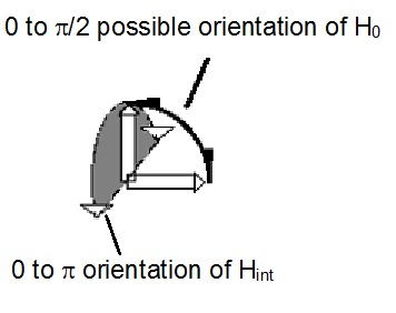
Fig. 1. Illustrating the possible orientations of the axes of magnetic field, H0 due to an orbiting charge (indicated by long arrows) and the internal field, Hint, due to “extra-bonding” valence electrons (indicated by shorter or broader arrows).
The additional internal field, Hint, is due to the coupling of the field due to the orbiting charge, H0, in essentially two-dimensional orbits (solenoid) with the spin, Sv. Because of the two-dimensional orbit, the internal field should be proportional to the spin density in two-dimensions (2D) which we take to be proportional to nv2/3, if we take nv to be a 3D quantity. When the magnitude of Sv is given by (Sv(Sv + 1))1/2, we obtain
Vµ Hintµnv2/3µ {S(S + 1)}1/3(17a)
or
V= CV{S(S + 1)}1/3. (17b)
The dimensionality arguments above for obtaining eqn 19a is consistent with that used by us8 to account for the binding energy, DH-H, of the (“ordinary”) hydrogen molecule. The , difference of ~Emaxexc/3 and between DH-H and maximum excitonic binding energy, Emaxexc» 6.8 eV has been attributed8 to a loss of a translational degree of freedom at the instant of bond formation in the one-dimensional chemical bond.
The term FS is then given by
FS = 1 + V = [1 + CV{S(S + 1)}1/3]. (18)
which is of the form found empirically. When we assume CV» 0.2, we obtain the calculated value FS(calcd) = 1.18, 1.25, 1.31, 1.36 and 1.41 for or S = 0, ½, 1, 3/2, 2 and 5/2, respectively, which is within 2% of that observed9, 58 empirically. It only remains to provide an estimate that justifies CV» 0.2» 2/p2. The involvement of p suggests a geometrical probability. We examine one possible explanation.
For obtaining the value of CV we do not need to consider the magnitude of the spin Sv or that of the magnetic field, H0, due to the solenoid. One requires the probability, p(orient), that the magnetic moment, m(nv), due to the nv “extra -bonding” valence electrons is aligned to H0 due to the orbiting charge (solenoid).We apply simple arguments from the Buffon needle problem that we have used20 earlier in the context of the magnitude of resistivity at the insulator-metal transition. In that communication we have examined the probability of two doublet valence electrons, ·, being converted to spinless charges, (··)– in the charge-transfer bond formation. These arguments are expanded upon later (see section ).
What is relevant as far as this communication is concerned is we interpret the term (2/p2) in eqn 12 as arising from the Buffon needle probability, p(= 1/p), of finding a particular orientation of the spin, Sv, of “extrabonding” electron, i, for one of two equivalent orientation pj½(= 2/p) of the valence electron, j, at any instant. The term 2/p2 is then obtained as p|= pipj½. We thereby obtain an expression for FS as
FS = 1 + p|{sv(sv+1)}1/3 = 1 + (2/p2){sv(sv+1)}1/3(19)
The above arguments would seem to apply to “charge-transfer” bonds. It is not clear whether they would apply to “neutral” bonds. There could exist more general arguments for the value of Cz that need not depend on whether there is charge-transfer or not during bond formation. A common thread could exist in the role of magnetic interactions informing, ignoring if there is currently
The point of interest is that independent of the “charge transfer” or “neutral” nature of the chemical bond, the axes of the magnetic fields, H0, H0e- and H0h+, determine the intra-atomic spin axis of the bonding valence electron, eo. The axis of the magnetic field, H0, may vary from 0 to p/2 (Fig 2). In the bonded state, the bonded pair of valence electrons may be considered to be spinless. Because of this one may consider the field, Hint, due to spins, Sv, of the nv “extra-bonding” electrons to be de-phased or decoupled from that of H0. If such a de-phasing was complete one would expect that CV = 0 and in its absence one could expect CV = 1. The consequence is that there is (Fig. 2) a canting of Hint away from H0 over all angles from 0 to p. Integrating over the canting angles as in the Buffon needle problem, we obtain z = 2/p2. This supports the contention that the dependence of FS on nv does not depend on the nature of the bonding in the “axle region.
A change by (1 + V) of the valence size will correspondingly lead to a reduction in the core size one the conditions for the classical turning point is maintained. We may therefore use33 the identify FS = (1 + V). It is known empirically from the way the correction FShas been applied in eqn 3 that the reduction in lengths with increase in bond order due to the “extra-bonding” valence electrons affects both the “ball” as well as the “stick” to the same extent.
In the above interpretation, the decrease in bond distances due to an increase in nvis not due to an increase in the number of bonding electrons in the bonding region in the sense that one writes, for example, C-C, O=O NºN, for single, double, and triple bonds, respectively..
The use of the concept of “extra-bonding” electrons to quantify bond order from experimental bond distances satisfies the criteria set by Jules and Lombardi89 that it should be “easily measurable”, with “few adjustable parameters”, “applicable throughout the periodic table”. In such a description the number of electrons per unit length in the bonding region is expected to increase purely as FS and would be less than the formal bond order given by (nv+ 1). This should satisfy the fourth criterion of Jules and Lomnardi89.
Inter-atomic distances in Elements
A straightforward application of eqn 7 to the inter-atomic distance in elements (Fig 1a) using values of rnZccalculated from the position of the element in the periodic table, and values of the number, nv, of “extra-bonding”valence electrons from refs 58 and 62 gives a fairly good fit between observed and calculated (eqn 7 with DMM =D0+ + D0– = 70.6 pm)inter-atomic distances with
dMM(obs) = 1.046(0.008)dMMmm+(cal)(0.994)(20)
We find that elements such as Mg, K, Ca, Rb, Cs, are greater than (see Fig 1b) the calculated values by ~ 2aH/3 or that DMM~ 2aH (instead of 4aH/3) which is close to the bond length of the elongated hydrogen molecule.

Fig 2. Plots of observed inter-atomic distances in elements at NTP vs the calculated charge-transfer distance parameters in Table 1 and eqns 6 and 7; straight lines are meant as a guide to the eye for various slopes. (a) Circles: Calculated using nominal valence states and number, nv, of “extra-bonding” valence electrons as indicated by the position of the element in the periodic table; actinides would have nv = 1 “extra-bonding” valence electrons like the lanthanides if the 5f electrons were localized; dashed line; slope = 1; straight line slope = 1.04. (b) Calculated distances from eqn 7 (FS = 1) for some p-block elements using rnZc values calculated from eqn 3for values of nval that could be different from that expected from the nominal values, nomval; straight line: slope = 1. (c) Showing nature of plot after changing values of nv (see Fig 3a)values for the transition metals and actinides, values of nval for some p-block elements, as well as the size of the “axle” to 2aH instead of 4aH/3. Dashed line slope = 0.02; fullline: slope = 1.
For the d-block elements, the divalent state, MII is usually taken to be the nv = 0 state. The value of nvis taken from the position of the elements in the periodic table, with a nominal dnv valence electrons and a nominal valence state of M(nv+2) with nv “extra-bonding” valence electrons. As the term “extra-bonding” implies, the nv electrons contribute to additional bonding, with the implication that these “extrabonding” electrons in the elemental metals are to be treated as electrons in a band with its attendant weak, Pauli-like paramagnetism. In the case of the transition metal elements the values of nv that is used in eqns 6 and 7 to obtain a reasonable fit with inter-atomic distances are given in Fig 3a. For the first half of the d-blockelements, good fits are obtained (except for Cr and Mn) using values of nv that is expected from the nominal values, nnom, as expected from the position of the element in the periodic table. Since nv is an atom-independent measure of shortening of inter-atomic distances through FS (eqns 6 and 7) one may expect the inter-atomic distances in d-block elements to contract universally with the value of nv. This is roughly what is observed (Fig 3b) once the distances are normalized at a particular d-electron number¾in this case at d3. For these metals there is a rough relationship between nv and strength of bonding¾such as heat of vaporization, DHvap¾and nv (see Fig 3c).
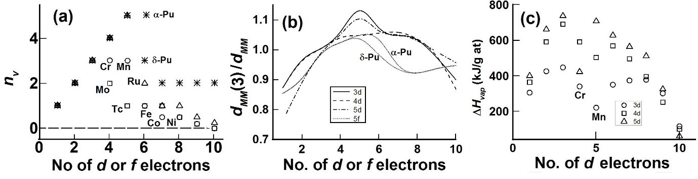
Fig 3. Changes in fitted values of nv,bond length and heat of vaporization, DHvap, with the nominal number of d- or f- electrons electrons. (a) Values of nv used to fit (in Fig 2a) inter-atomic distances, dMM, in elements for 3d- (circles), 4d- (squares), 5d- (triangles) and actinides (stars). (b) Variation of the inverse of inter-atomic distances, dMM, normalized to that, dMM(3), of the element with nominal d3 or (d + f)3 configuration; the lines give aB-spline fit. (c) Changes in DHvap per g atom of element for d-block elements.
When nv is less than nnom, the nominal number of unpaired d electrons from the position of the element in the periodic table, then there is likely to be nloc(= nnom – nv)localized electrons which contribute strongly to magnetic properties. The low-temperature itinerant electron antiferromagnetic behavior in chromium and manganese is consistent with the existence of localized electrons withnloc= (nnom – nv) ~ 1 and 2 for Cr and Mn, respectively (Fig 1a). The complex crystal and magnetic structure of a-manganese76-79, show that atoms at various sites in α-Mn have different localised magnetic moments and Mn-Mn distances. Mn has a cubic unit cell with a lattice parameter of ~ 891.5 pm with 58 atoms per unit cell. The average volume per Mn atom is ~ 230 pm3 so that the average Mn-Mn distance is taken as ~ 230 pm. In the refined structure. The longest Mn-Mn distance (site I) is between 284 pm and 272 pm; this site has the largest magnetic moment of ~ 1.9 mB. The shortest Mn-Mn distance (~ 225 pm) is between Mn atoms at sites III and IV; the magnetic moments at these sites are between 0.60 mB and 0.25 mB. The calculated Mn-Mn distances for nv = 0, 1 and 3 are, respectively, 301 pm, 254 pm and 229 pm, respectively. One may expect from our model, therefore, that nloc is between 4 and 5 for site I and close to 2 for sites III and IV. The trends between the observed moments and nlocis therefore consistent. The discrepancy between the observed localized moments and nloc may be attributed to itinerantantiferromagnetic character.
The ferromagnetic behavior in Fe, Co, Niis also consistent with the existence of localized electrons. The saturated magnetic moments, MS of the ferromgneticsystems are somewhat less than nloc. This is expected when we interpret Stoner’s model in terms of an itinerant electron ferrimagnetism¾anda term coined66,67 recently¾with at least (nv + nloc – Ms) electrons being itinerant and a maximum of nloc electrons being localized.
In the case of the nominally d9 metals, Cu, Ag, and Au, the fit of calculated distances using rnZcvalues for the nominal divalent states requiresnv<1. This would require the existence of localized electrons which is inconsistent with their diamagnetic properties. A better fit is obtained with the distances calculated using rnZcvalues for the nominal monovalent states and nv = 2 (MI2) . The ratio of observed/calculated values for MI2 (values in parentheses are for MII1) are Cu 0.97 (1.094), Ag 1.01 (1.13) and Au 0.96 (1.068).
In the Lanthanide elements nv = 1 for all the lanthanides except for Eu and Yb which are better fitted with nv = 0. This is consistent with the findings70-72 that Eu and Yb are in the divalent states and that the other actinides are in trivalent states with the 6s2 and 5d1 electrons being itinerant. The 4f electrons are not “extra-bonding” and therefore are to be treated as localized.
In the case of actinide elements (starting with actinium) the trend in the values suggest that the actinides mimic the behavior of other d-block elements as proposed72 quite early.The admixture of 5f and 6d states is likely in this case so that in the initial stages one expects nv = n5f + n5d so that the early 5f electrons are itinerant, and one cannot really distinguish from our analyses whether the identity (5d- or 5f-) of the band electrons. In the case of plutonium the nominal value, nnom, of 5d+5f = 6. We find (Fig 2) nv = 5 for a-Pu (av Pu-Pu distance ~ 305 pm calculated from the ~19% decrease in volume from d-Pu) taken to be and nv = 3 for d-Pu (dPu-Pu = 328 pm) so that nloc = 1 and 3 for the a- and d-phase, respectively. RecentlySöderlind et al71find from DFT calculations that there is an f-band participation.They noted that for plutonium the 5f are on “the edge between localization and itinerancy”.The growth of the fine structure70, 83 of the XPS or UPS spectra on going from U (absent) to a-Pu and being clearly visible in d-Pu and well removed from the Fermi level in Am shows localization of f-electronsis mainly complete with Am. Changes in the branching ratio of the M4,5 (3d→5f) EELS (electron energy loss spectroscopy) edge as is sensitiveto changes in the environment of the actinide element, exhibiting decreasing changes in the branching ratio with localization.The largest difference in branching ratio between ground-state actinide metal phase and actinide dioxide from Th to Cm is seen for Th and U, with no difference for Am and Cm, thereby showing70 that localization of f- electrons is nearly complete with Am.
After the above considerations, the best linear fit with zero intercept between observed and calculated distances give (Fig 1b)
dMM(obs) = 1.020(0.003)dMMmm+ (cal) (R = 0.999) (21)
The elements Zn, Cd, Hg show a consistently larger value when we calculate with nv = 0 and nval = nnom = 2. This could suggest that an admixture of the monovalent state with nval = 1.
Influence of Metallicity in Elements
An important issue that is not considered in the context of metallicity of elements is the separation of spin- and charge-degrees of freedom. This issue has become relevant in the context of metallic non-fermi liquid behaviour in high-temperature superconductors. In a Fermi liquid metal, the spin and charge degrees of freedom exist together which we have interpreted20in the simplest t-J model (t = transfer integral, J = exchange integral(= 4t2/U is assumed in most theoretical treatments, U being the correlation energy)as meaning that the time scales of defining a spin by its Larmor precession period, tLint(= 2h/zJ), due to an internal exchange field, Hexch(= 2zJS/gmB,zbeing the nearest-neighbour coordination number), of another atom, is less than the residence time, tW(=h/2zt, for a bandwidth W= 2zt in the tight-binding approximation), of an electron at a site. We then obtain
tW / tLint= J/4t = Pt/4U. (22)
As the transfer integral increases for a fixed value of the correlation gap U, we have two limits (from Eq. 22)
- i) Pt /4U> 1. From Eq. (22) tLint<tW, such that the spin of the electron is well-defined by its internal Larmor period, tLint, for the time defining the charge at a site. The spin excitation gap is smaller than the bandwidth. The Mott-Hubbard criterion125 for metallization, Wb³ 2U is satisfied for z³ P/4 such that even z = 1 (as in a chemical bond) satisfies the Mott_Hubbard criterion for metallization.
- ii) Pt /4U< 1 J/t< P/4 and tLint>tWunder these conditions. The residence time of a charge-carrier at its site, tW (defined by t), is less than the J-dependentLarmor precession period, tLint. The direction and/or magnitude of the internal field, Hexc changes with every t-dependent transfer of the spin-less charge. The spin-excitation gap is larger than the bandwidth in such cases. An itinerant electron state in which there are sites with Pt/U < 1 (for same values of z)would have slower relaxation dynamics for spin as compared to charge. Because of this, such systems may behave as non-Fermi liquids.
The above criteria holds for systems containing at least two atoms so that a transfer integral, or a bandwidth is defined. One could assume that in the case of bonds between insulating elements, the condition tLint>tW holds so that constraints acting on the spin would be operative. In the case of bonds between metallic elements the condition tLint<tW holds the constraints due to the spin of the electron need not be operative within the life-time, tW, of the charge of the electron. The most important of these constraints is the constraint on spin-conservation in a “charge-transfer” bond when spin-less charges are created from pairs of doublet electron. We have argued that the values of the coefficients C+ (= p2/3 ~2.145) and C– (= p4/3/2 ~ 2.301) (Table 1) arise because of these spin-conservation constraints. It turns out (see section ) that these coefficients are applicable to three-dimensional solids in general even for metallic elements, as we have seen earlier (see section ), as also for solid salts of metallic elements¾e.g., solids with rock-salt structure.
Of particular interest is the classical problemfirst discussed127 by Born andHeisenberg in 1924, of the “expansion” of M-X distance in alkali metal halides when condensedinto a solid as compared to that in the gas-phase. Such an expansion is notnecessarily related to the importance of repulsive terms in solids126. The gas-phase distance is actually a contraction relative to that in crystals for alkali metal halides the best fit gives
dMX(obs)(cryst) ~ dMX(obs)(gas) + aH (23)
with R factor ~0.99). On comparing eqns 23 and eqn 5, there could be a suggestion that the gas-phase M-X distance in MX alkali metal halide monomers is a “charge-transfer” bond with DMX = aH/3 or that CR0– = aHinstead of 4aH/3 or 2aH, respectively, (Table 1). Such a trend is not observed, however, for the gas-phase distances in halogen molecules. As compared to those in solid halogens. There is a contraction in gas-phase M-M distances in alkali metal dimers as compared to the corresponding solids. The contraction does not follow eqn 23, however. We have shown in Fig 4 a comparison of observed M-M distances in solids (filled circles) and gas-phase dimers (circles with cross) vs the calculated “charge-transfer” distances dMM00± (see eqn 7, FS = 1, Table 1)for the alkali metals. The gas-phase dimers show the “contraction” in M-M distances relative to that in solids even though the bonding is not expected to be “ionic”. The dimer distances are indeed considerably shorter than “charge-transfer” distances.
The dimer distances are best fitted by “neutral” values of CMCMDMM as indicated by values in the box. It is seen that fractional “neutral” values of CM,Xare used to fit dimer distances besides the restricted values given in Table 1. A feature that we encounter elsewhere (see later) is that the values of CM,Xas well as DM,X used to fit observed M-X distances increase with increasing values of rnZc(M,X), especially in isolated dimers.At the same time, the M-M distances in solids are considerably larger than the calculated values of dMM00± in the case of Na, K, Rb and Cs. The distances in the solids are well fitted to observed values (for zero intercept, R > 0.999) by the following CMCM’DMM” values (in brackets):Li (224/3), Na (222), K,Rb, Cs (pm2) with slope of 1.033(0.013). Of interest is the admixture of “neutral”and “charge-transfer” values for the “ball” and “stick” sizes. We discuss this aspect later. Before we do so it is important to examine a single atom criterion for metallicity instead of the essentially two- (or more-) atom criterion in eqn 22.

Fig 4. Plots of observed M-M distances for alkali metals versus calculated distance, dMM00± (nv = 0), in dimers (circles with cross: dimers) and solids (filled circles). Thin full straight line is meant as a guide to the eye for the correct fit. Symbols in the box represent “neutral” CM,CX,DMX (see eqn , M = X) values for fitting the distances in gas-phase dimers (Broken line shows goodness of fit).
The question of whether a single atom criterion for metallicity in elements may exist may be considered to be incomplete as by its very nature a metallic substance is judged by its bulk properties, especially its ability to conduct current without barrier to charge transport or without activation. This criterion if it exists at all must be connected related to the proximity of an excited state and hence is expected to berelated, first of all, to the dielectric polarizability, a. Alternatively, there could be a screening length, akin to a Debye-like screening length, lD, such that an atom, M, with sizes rnZc(M) >lD would be metallic.
The importance of the polarizability, a, for understanding the metallization process in solids has been emphasized in the Herzfeld–Goldhammer theory111-113. The Herzfeld criterion is expressed in terms of the Clausius-Mossotti relationship between the index of refraction, n (high-frequency dielectric constant), e, the atomic refractivity, R, and the atomic volume, Vm.
(n2 – 1)/( n2 + 2) = (e – 1)/(e + 2) = R/Vm (24)
When R/Vm = 1, the Clausius-Mossotti relationship is satisfied only when e®¥. The divergence of the dielectric constant has been termed as a “dielectric catastrophe” by Mott[5]. In this case the excitonic binding energy of a charge-carrier to its hole will vanish and the charge-carriers will be free. Metallic elements have R/Vm³ 1 at NTP thus satisfying the Herzfeld criterion. There has been the question as to whether there is an intrinsic single-atom property that allows a distinction to be made between insulating and metallic elements. The Herzfeld criterion111,112 is really based on interaction between atoms and an imminent polarization catastrophe as the concentration is increased.
The second criterion is due to Mott108 who examined a potential, V(r), around a positive charge which is of the form
V(r)= −(Ve2/er)exp(−lr) (25)
wheree is the dielectric constant of the medium and V is the nuclear charge. Eqn 25 is known as the Debye-Hückel potential in plasma physics and is known as the Thomas-Fermi or screened Coulomb potential in solid-state physics and atomic physics when the potential is applied to a degenerate charged fermion system. A test charge in electron plasmaappears neutral108,119-121 due to screening at a distance r >lD. The concept of a Debye screening length in plasma describes in general the important phenomenon of electrostatic screening in many different areas. Charge separation exists in plasma for distances smaller than the Debye length while at larger distances from the charge the plasma is quasi neutral. For a typical electron density in metals lD(~ 1 Å) <lF (~ 5 Å) the Fermi wavelength, so that lD has not been used as a criterion for metallicity in elements118. However, for atoms118 the de Broglie wavelength is smaller than lD and an atomic-size criterion may be used.
Mott proposed108 that due to the dielectric screening, the attractive electron-hole binding energy in a doped semiconductor is decreased due to a screening by other charges over a screening length, l. The potential V(r) of eqn 23 does not give rise to a bound state for a critical value, nc, of the dopant when lbecomes large enough such that the potential becomes too small for a bound state to form because of the screening of the long-range Coulomb potential. Mott proposed that the critical value of ncis given by nc1/3aHexc» 0 where aHexc (= eexcaH) is a dielectric-constant-dependent excitonic Bohr radius, eexc being the dielectric constant. Mott’s idea108 of estimating dopant concentration at which doped semiconductors become metallic, uses a single-site Thomas-Fermi screening length, lTF (>l, the de Broglie wavelength4), with a charge appearing neutral¾and therefore free of any localizing electrostatic potential¾at distances greater than lTF (>> lattice spacing) from the dopant.The Thomas-Fermi screening length, lTF, of the valence electron when a charge appears neutral at distances greater than lTF from the dopant has been used as a single-site estimate of dopant concentration at which doped semiconductors become metallic108.
For a typical electron density in metallic elements lTFis not a discriminating criterion since lTF(~ 1 Å) <lF (~ 5 Å) the characteristic Fermi wavelength for electrons. For heavy nucleons or ions the screening length118-121 is greater than the characteristic de Broglie wavelength. Both the Herzfeld (volume- or interaction-dependent) and Mott (screening-dependent) criterion are concentration-dependent and is not a single atom criterion for an isolated atom.
In Mott’s model of screening the excitonic Bohr radius aHexc is usually much larger than inter-atomic spacingsuch that a single-atom criterion for metallicity is not prompted by Mott’s model. It is known, however, that for the ground state of hydrogenic atoms with nuclear charge, Z,in a classical plasma the energy goes to zero for l ~ aH/Z [29, 30]. The screening length in this case would be much less than typical bond lengths or inter-atomic distances. One could then use a core atomic size for distinguishing between insulating and metallic elements. Because of the inevitability of a perceived many-atom requirement to account for metallic behaviour, there has been little emphasis on finding a relation between any size of an atom and a screening length that provides a single-atom metallic criterion for metallic behavior. The earlier attempt8 to distinguish insulating elements from metallic elements required that rnZc> 2aH/3 ~ 0.67a u at NTP was not quite successful (Fig 5a) in clearly separating metallic elements from insulating ones.
A connection has also been sought136 between polarizability, a quantifiable quantity, and electronegativity, first defined famously by Pauling132 as “… the power of an atom in a molecule to attract electrons to itself” and now left hanging midway in the gap between occupied and unoccupied states133, 134. In a sense, the electronegativity is inversely related to the on-site correlation energy, U, which in a Pauling-like way may be looked upon as the power of an electron to repel another electron from itself. One expects, therefore, to find a limiting value of the electronegativity that separates insulating elements from metallic ones. Both the electronegativity scale, cP (Pauling), as well as the dielectric polarizability radius, ra, for atoms have been related to a core atomic size. There is a critical value for both these properties that separates insulating elements from metallic ones (at NTP), that enables one to examine evidence for a screening length, lDmet.
The core sizes <rnZc> and {rnZc}* are linearly related12 to static electric polarizability radius130,131,136, ra, and the inverse of Pauling’s electronegativity, cP-1, respectively. These sizes are given by11, 12
<rnZc>(h) = 1/nval + (aH/2)ln{(ZRG(h-1)/nval)1/3} (26)
{rnZc}*(h) = 1/nval+ 0.5(aH/2)ln{(ZRG(h-1))1/3} ~ cP-1(27)
where, nominally, h is the principal quantum numbers for elements, nval is the number of valence s-and p-electrons and ZRG(h-1) is the number of electrons with rare-gas configuration with principal quantum number (h -1). The Pauling electronegativity, cP, is found to be ~ [{rnZc}*(h)]-1. The polarizability radius, ra, is found to be given by
ra(M) = ea(4p/3)1/3{(2<rnZc>(M)) + eaHi,maH} (28a)
= ea(4p/3)1/3r’a(M) (28b)
(((4*3.1416)/3)^0.3333)*(2*col(avrnZc) + 52.9)
with
r’a(M) = {(2<rnZc>) + aH} (29)
The value for the effective dielectric constant, ea, may be different from eMX in eqns 5 or 7.We find that the coefficient, eai,m, for aHin eqn 28a depends on whether the atom is that of an insulating or metallic element. From the fits we find for metallic elements eam = 1; for insulating elements an atomic-size-dependent expression for ea may be used with
ea = 1 + (3/4p)r’a3/rvdW3 (30a)
= 1 +r’a3/(4prvdW3/3) = 1 + a’/Vatom (30b)
where r’ais obtained from eqn 29 and rvdW is a size associated with a neutral isolated atom which we have taken as a van der Waals’ radius given by (see later)
rvdW= 1.15(2.3rnZc + 2aH) »{(p8/3/8)rnZc + 2aH} (31)
The interpretation of the term 3/4p in eqn 30a is unclear. We have included it in the volume Vatom = 4prvdW3/3 in eqn 30b. Thus for insulating elements we write
ra(M) = ea(4p/3)1/3{(2<rnZc>(M)) + eaaH} (32)
For transition metals we use the expression
ra(M) = ea(4p/3)1/3{(2<rnZc>(M))/FS(M) + aH} (33)

Fig 5. (a) Plots of the atomic size, rnZc (from ref 11) vs atomic number, Z, for elements upto Z = 118 (uuo); open circles: insualting elements (at NTP); partially filled circles: metallic elements (at NTP). (b) Plots of {rnZc}*/Fsvs<rnZc>/FS (eqns27, 28) for the elements, FS calculated from eqn 6 using nv values from Fig 3a; meaning of symbols indicated in box. Inset: Plots of experimental polarizability radius, ra (expt), obtained from tabulated experimental values of the polarizability, a (ºra3) vs the calculated polarizability radius using eqn 26a for non-transition metal atoms and eqns 32 and eqn 33 for transition metal atoms. Circles: from ref 131; filled circles: rare-gas, alkali metal and Al, Zn, Cd and Hg atoms: triangles as tabulated in ref 137. The values for Uranium correspond to scalar (sc) and static (dc) polarizabilities(from ref 138). Best fit (shown by dashed line) gives ra(expt) = 1.000(0.010)ra(cal) (R > 0.996, SD < 8 pm)
We have shown in Fig 5b the plots of the calculated values of {rnZc}*/FSvs<rnZc>/FS for all the elements using eqns 26 and 27 and with nv = 0 for the transition metal elements. It is seen that in this case there is a clear demarcation between insulating and metallic elements for both {rnZc}*/FS and <rnZc>/FS at aH/2. However, if we take nv values as Moreover, since < rnZc>» [2{rnZc}* – aH/2] (Fig 1) for insulating elements, a sought relationship12 between cP-1 and ra is suggested.
The numerical solution116 of the Schrödinger equation for hydrogenic atoms with a nuclear charge, V, and interacting through a Debye-Hückel-Yukawa screened potential gives a screening length l = 0.84aH/DoV for 1s orbitals (Do ~ 0.78)when the binding energy goes to zero. This would imply that V» 2 when lD = aH/2. A Bohr size h/meffe2 = aH/2 is obtained for a light negative charge of mass 2me (me = mass of free electron) as in hookium192-194 or spherium195. We write an interaction between two hydrogenic atoms, Åe–, at sites A and B as
(Åe–)A + (Åe–)B « (Æe)A + (Åe–)B« [ÆeÅ]e–« [ÆÅ](ee–) º¨+(ee)– (34)
whereÆe is a neutral charge-less pair, as appearing to an external charge because of screening. When ÆeAand Åe–B pair form a composite particle ¨+(ee)–, attractive (electronegative) electron-nuclear interaction in Æe and also Mott-Hubbard repulsion16 between electrons in (ee–) is overcome. The value V = 2 could come from the coalescence of two Å nuclei on the LHS of eqn 34 to form the Æź¨+ nucleus; the ee–pair with mass 2me in the hydrogenic-atom like ¨+(ee)– in the RHS of eqn 34would be equivalent to V = 2 for the nuclear charge. satisfying at the same time the condition for constant m = 0 chemical potential for rnZc as well as the sizes contributing to dMX.
The single atom property separating insulating from metallic elements when <rnZc>/FS = aH/2 isra ~ 171 pm from eqn 32 and eqn 33 when approaching from the metallic side (ea = 1). This is an experimentally verifiable quantity. The tabulated values of the polarizability radius across a metal-insulator transition in the elements across a row in the periodic table shows such a trend. Thus we find (metallic elements in bold and polarizability radius from the literature136, ra in brackets) the following:- Be(178)/B(145), Al(203)/Si(175), Ga(201)/Ge(182), Sb(188)/Te(177); Po(189)/At(182). If we calculate ea from eqns 30, the calculated values of ra(liter)/eawhen becomes the following:- Be(171.2)/B(141), Al(195)/Si(170.2), Ga(194)/Ge(175.3), Sb(183)/Te(172.5); Po(176)/At(167).
The issue that has come to the fore in the context of recent exposure to developments in areas such as high-temperature superconductivity, magnetoresistance is the nature of the metallic state and especially the question of whether the metallic state is a Fermi liquid or not. Early descriptions of the resistivity of metals tacitly assumed that the metal behaved as a Fermi liquid. This aspect becomes critical when we examine the metallic nature of an element by the magnitude of its resistivity and not by the temperature-dependence of the resistivity.
As one approaches the metallic state from the insulating side, barriers to transport become vanishingly small.In terms of chemical reaction rate theory the approach to metallization is perhaps equivalent to the approach to fast barrier-less charge transfer reactions, when reaction cross-sections become large compared to local structural parameters. Once such a state is reached, the actual microscopic chemical nature such as the identity of the element, or its ionization potential or electron affinity or correlation energies may not be relevant. Instead, one may consider the precursor to the metallic state as a dielectric continuum in which the charge carrier bound to its hole, which we consider to be an exciton, and not necessarily a photo-excited particle. The band gap of a semiconductor is, by definition, the energy necessary to create an electron (e–) and hole (h+) at random with respect to the lattice and far enough apart so that the Cooulomb attraction is negligible. If one carrier approaches another they form a bound excitonic state approximately described by a hydrogenic Hamiltonian with an energy slightly below the band gap. The effective masses of the two carriers are often only a small fraction of the electron mass.The binding energy of the exciton, Eexc, is determined by its Bohr radius and dielectric properties of the medium through its dielectric constant, e. Itis given141 by Eexc = me4/(h2e2) where m is a reduced mass. The process of electrical conduction is then by excitation of the excitons by an energy Eexc to electron and hole charge carriers and then charge-transfer from one charge-carrier-site to another in response to an electric field.

Fig 6. Plots of the electrical resistivity, rvs {rnZc}*/FS (from eqns 27 and 6) using nv values from Fig 3a for transition metal elements. Circles: insulating elements; Partially filled circles: metallic elements.
Ganguly20 has pointed out that if one considers the conductivity to be a measure of the probability of charge transfer and relate it to the probability of coherent or resonant excitation energy transfer then the in this excitonic picture the electrical conductivity may be written as
sexc = Eexc/h (35)
whereEexc is the excitation energy of an exciton with Bohr radius aHexc. If we consider charge-carriers in an energy band of width Wb, and with an energy EW at the top of the band, the charge carrier will be free of all attractive binding potential which have an excitation energy Eexc<EW. Eqn 35 is an expression of this constraint for a coherent excitation or energy transfer.The non-interacting electron gas of the metallic free electron Fermi liquid state is treated as a high-energy or high-temperature state with the energy of the charge carrier being larger than Eexcmax, the maximum possible energy for any binding or localizing interaction of a charge carrier to its hole. The maximum binding energy141-143, Eexcmax ~ 6.8eV, corresponds to e = 1 and the reduced mass m= mo/2 where mo is the mass of the free electron.
It could be assumed that when the charge carrier has energy, EW, greater than Eexcmax it will be free of all attractive binding potential to its hole and would then behave as a free electron gas of the kind to which Fermi liquid theory is applicable. The minimum conductivity, smin(FL), of a Fermi liquid is then given by
smin(FL) = Eexcmax/h = m0e4/4h3 = e2/4haH» 6.8 (eV)/h (36a)
»11,360 S cm-1
yielding a maximum resistivity, rmax(FL), for the Fermi liquid as
rmax(FL) » 88 mohmcm (36b)
The electrical resistivity of the metallic elements near room temperature144 are mainly below rmax(FL) (eqn 36b) or close to it. Manganese has a resistivity slightly larger than rmax(FL) which could be consistent with the existence of localized electrons as discussed earlier. All the elements characterized as insulating have r>rmax(FL) except for As, which has {rnZc}* ~ 0.44 for the nominal value of nval = 5 from its position in the periodic table. At low temperatures the electrical resistivity of arsenic along its binary axis shows146,147 reaches values as low as 10-7ohm cm (<rmaax(FL)) and shows T3temperature-dependence over two decades of temperature somewhat atypical of Fermi liquids (T2 dependence). The basal plane As-As distance of nearly 250 pm in rhombohedral As is better fitted by AsIII (Fig 2b) with nval = 3 and {rnZc}* = 0.574 a u >lDmet= aH/2. The out-of-plane As-As distance of ~ 314 pm is close to {(2CR0–(As) + dAs–As00±)/2} ~304 pm for AsV than to ~ 336 pm for AsIII. Arsenic may therefore be looked upon as a 2D FL metal. It is not superconducting146,147 as in the over-doped superconductors.
In the case of polonium, the electrical resistivity is reported to be between143,144 40 mohm cm (<rmax(FL))and 174mohm cm (>rmax(FL))around room temperature which suggests that polonium is at the border line of being a Fermi liquid. The value of {rnZc}*(PoVI) is 0.499 a.u. which is just at the borderline of metallicity while {rnZc}*(PoIV) ~ 0. 582 a u which is well into the metallic state. The Po-Po distance in the simple cubic structure of a-Po is best given by PoIV with DPo-Po = 2aH in eqn 7 (FS = 1). It is not clear to what extent the admixture of PoVI and PoIVinfluences coherent electrical transport. It is known, for example, that below the ferromagnetic transition in mixed-valent manganites such as (La, Sr)MnO3, there is metallic behavior at low temperatures at ambient pressure while the high-temperature phase is insulating. The trigonal structure is obtained by an elongation or contraction along the <111> direction of the simple cubic structure. The transition from the high-symmetry cubic a-Po to the distorted lower symmetry b-Po with increasing temperature is counterintuitive since high temperatures usually favour higher symmetry. This distortion is thought to be due to a Peierls instability152, spin-orbit coupling150, 153, 155, or the separation154 of s- states from the p-states, so that the purely right-angle bonding sustains the simple cubic structure of a-polonium. In the context of metallization, one may argue that low temperatures favour coherent transport in, say, Bloch-like states with Fermi temperatures, TF> Tdist, the distortion temperature. At higher temperatures, Fermi liquid character disappears and only the distortion remains. More elaborate experiments on difficult-to-study polonium would be required around the a-b transition.
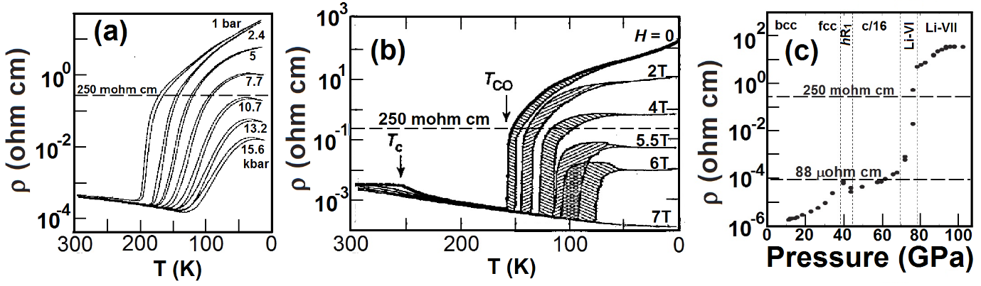
Fig 7. (a) Plots of resistivity vs temperature for NdNiO3 at various pressure (from ref 190, see also refs 188 and 189). (b) Plots of resistivity vs temperature for Nd0.5Sr0.5MnO3 at various magnetic fields and ambient pressure (from ref 181). (c) Plots of resistivity vs temperature for lithium at various pressure and 25 K (from ref 161).
One of the more intriguing feature in recent times is the transition161 of Li metal from a metallic phase at ambient temperature to an insulator at high pressures (around 85 GPa) both by resistivity measurements as well as by reflectivity measurements. Since {rnZc}*(Li) ~ 1.03 a u >aH/2 one expects the Li metal to be a Fermi liquid (Fig 6) with a resistivity r<rmax(FL) ~ 90 mohm cm which it is at ambient pressure. However, at higher pressures the resistivity increases by more than four order of magnitude and is well above rmax(FL).
In order to obtain a better perspective on this transition we have compared the changes161 in the resistivity of Li as a function of pressure (Fig 7c) at 25 K with that of perovskite oxides such as190 NdNiO3 (Fig 7a) as a function of temperature at various pressure and that181 of another perovskite, Nd0.5Sr0.5MnO3, as a function of temperature at various magnetic field, H(Fig 7b). The effect of increasing pressure on Li at 25 K is, resistivity-wise, similar to the effect of decreasing temperature on the perovskite oxides. The effect of increasing pressure on NdNiO3 at low temperatures (Fig 7a) is to drive r towards rmax(FL) or below it; in the case of Nd0.5Sr0.5MnO3, r decreases with applied magnetic field towards rmax(FL) (Fig 7b). This effect of increasing pressure or increasing magnetic field is in the direction of lower resistivity which is what is conventionally expected. What is common in all the three examples in Fig 7 is that the resistance in the semiconductor region has a negative TCR (temperature-coefficient of resistance) typical of semiconductors as long as r> 250 mohm cm which we consider (see Fig 2 of ref 191) to be the maximum resistivity, rmaxNFL for a dirty metallic non-Fermi liquid state (this has been obtained from considerations of the lowest excitonic binding energy at the relativistic limit, rmaxNFL ~ afp8/3rmax(FL) ~ 250 mohm cm, with af being the fine structure constant). Li is truly not a metal at the pressures (around 85 GPa) studied by Matsuoka and Shimizu161.
With increasing pressure the structure of Li changes158 from bcc at ambient pressure through fcc to a distorted hexagonal phase at around 40 GPa with c/a ratio of ~ 2.25. Mercury, wih rnZc(Hg) ~ 1.05 a u close to 1.058 a.u. for rnZc(Li)has a similar structure with a similar c/a ratio. At higher pressures, after the metal-insulator transition, the density pressures is ~ 4 times more than the density at ambient pressures. Structural details and the phase diagram with increasing pressure are being worked. In anThis suggests a decrease of the ambient nearest-neighbour inter-atomic distance (~304 pm) to 304/41/3 ~ 192 pm. This distance is considerably larger than the shortest Li-Li distances in the high-pressure structure. A transition to the insulating phase with short- and long- Li-Li distances at high pressures due to a Peierl’s instability is sustainable, however. The so-called semiconducting L-VII C2cb-40 structure is a layered …ABCA”B”C”… structure perpendicular to b-axis, with174 shortest intra-layer Li-Li distance of ~ 160 pm and shortest interlayer Li-Li distance of ~ 178 pm. If we use rnZc(Li) = 1.058 au as tabulated in ref 11 the smallest all-“neutral” distance dLi-Li112 distance is ~ 217.8 pm while the mixed (“neutral”core and “CT” axle) distance, dLi-Li114/3 = 182.5 pm. These distances are much larger than the smallest Li-Li distances observed in Li at high pressures, say in the semiconducting L-VII phase. One would require smaller values of rnZc(Li) than that tabulated earlier11.
Neaton and Ashcroft163 noted that with increasing densities there could be increasing overlap between core electrons thereby reducing the relative volume of the valence electrons. This leads to a narrowing of the band and the crystal structure becomes unstable to a Peierls-like instability with even number of electrons per unit cell that leads to an opening of a gap and insulating behavior. Rephrasing these arguments Feng et al171 suggested that a new paradigm may be used to account for increasing localization under pressure by using the effect of orthgonality due to Pauli Exclusion Principle which would make the core electrons repulsive to valence electrons. The relative volume of the cores increase and force the valence electron to be localized in interstitials.
Our methodology11 for obtaining rnZc from the nominal electronic configuration of an atom (e.g., 1s2,2s1 for Li)does not depend directly on pressure. It may, however, take into account effects of any conjectured change in the electronic configuration from the nominal one. The critical feature that we must reconcile with in our model of screening length and metallicity, is the possible ways by which one gets an insulating phase in Li in the sense that we obtain a core size of lithium that is less than aH/2 or 0.50 a u. At least a two-atom property, such as dMX, is required to recognize screening effects since a charge appears screened only to another particle in the same medium. Because of this one could propose a two-atom criterion for a screened behavior involving an M-X linkage
{rnZc}*(M) + {rnZc}*(X) ³aH (37)
Valence electrons of M-X compounds which do not satisfy have been considered to be “static” while those which satisfy eqn 37 have been considered to be “peripatetic”. We shall use this terminology hereafter. Since {rnZc}*(Li) ~ 1.03aH it would seem that all linkages in any Li-X bond, including LiH ({rnZc}*(H) = 0), would be “peripatetic” and may not sustain charge-separated “hub” sizes in isolated LiX linkages. The condition of eqn 37 does not mean that the solid LiX compound should be metallic for “peripatetic” linkages. On the other hand, for “static” MX linkages, it is likely that MX would be insulating. In order that elemental Li should be insulating, it would be necessary that an excited state of Li, formed under pressure, would have a “static” Li-Li linkage (does not satisfy eqn 37).
We follow the thread of the arguments of others163, 171 and suggest that the route to a smaller value of rnZc (Li) is by an excitation of inner-shell electrons (1s2 electrons in the case of Li) to the valence state to give, say 1s12s2 configuration with two electrons in the valence shell (nval = 2, ZRG(h-1) = 1 in eqn 3), which we write as Li2*. The Li3* state is the configuration in which 3 electrons occupy degenerate 1s and 2s state (nval = 3, ZRG(h-1) = 0 in eqn 3 so that there is no core contribution). For these states we obtain from eqns 3 and 27 the sizes rnZc(Li2*) = 0.50 a.u. = {rnZc*}(Li2*) and rnZc(Li3*) = 0.333 a.u. = {rnZc*}(Li3*). From these changes one may expect elemental lithium with Li3* configuration to be insulating simply because eqn 37 is not satisfied. The {rnZc}*(Li2*} ~ 0.50 a u would just satisfy eqn 37. The “charge-transfer” Li2*-Li2*, dLi2*-Li2*00± distance of ~ 189 pm distance is consistent with a reduction in density by four times in the insulating phase at high pressures.
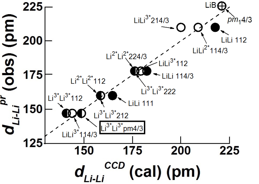 Cr
Cr
Fig 8.Plots of observed158 values Li-Li distance (210 pm around 45 GPa and theoreically modelled158 distances of 147 and 169-179 pm in the ‘paired-atom’ Cmca-like Li-oc8 phaseas well as observed134 distances of ~ 160 and 178 pm in L-VII phase at ~ 85 GPa in elemental lithium at various pressure vs the calculated distances using various CMCM’DMM’values as indicated against each point and rnZc values of 1.058 a.u. for Li (ref 11) and 0.5 a.u. and 0.33 a.u., for Li2* and Li3*, respectively (see text). Filled circles: calculated Li-Li distances; half-filled circles: Li3*-Li3* distances. Dashed line is meant as a guide to the eye for the correct fit. The observed178 and calculated, dLiB01± (nv = 1 for B) values of LiB is also includedin the figure.
We have shown in Fig 8, the calculated Li-Li distances using various CMCM’DMM’ distances using rnZcvalues for Li (1.058 a.u. from ref 11) and Li2* and Li3* discussed above. The shortest Li-Li distance with rnZc(Li) is dLiLi111(~ 165 pm) and involves a very low value of DLiLi = aHimplying a double occupation of the first Bohr orbit. Such a size would be our speculated size of hookium or spherium from the discussion on eqn 34. Calculations on lithium metal at high pressures does not show evidence for such particles although electron localization function analysis show the presence of doubly occupied sites at interstitials. The other short Li-Li distance with rnZc(Li) is dLiLi114/3 (~ 183 pm). Our analysis (see later) of gas-phase M-X distances do not show evidence for dMX111 or dMX114/3. The shorter distances of ~ 147 pm (calculated) or 160 pm (observed) require excited Li2* or Li3* sizes (Fig 8).
Among the alkali metals, only Li and Na show evidence161,168 for a transition to an insulating phase at high pressures. The high-pressure transparent phase of sodium with the hP4Crystal structure (space group P63/mmc) has Na-Na distances of ~ 188-193 pm which is close to the calculated dNa-Na114/3 distance of ~ 194 pm using rnZc(Na) = 1.192 a.u.. A “charge-transfer” pm4/3distance close to 193.6 pm ha is consistent with a c-axisof ~ 387.3 pm of he hp4 phase, a high band gap and a transparent nature would require rnZc(Na) ~ 0.523 a.u. The excited Na3* atom with two core electrons excited to the valence shell and eight inner-shell electrons (ZRG(Na3*) = 8) would have rnZc(Na3*) = 0.507 a.u. when x = 0.5 in eqn 3 and {rnZc}*(Na3*) ~ 0.38 a.u. This would make Na3+ well into the insulating phase consistent with its large band gap and its transparency162.
The values of rnZc(Li) = 1.058 a.u. and rnZc(Na) = 1.192 a. u. have been obtained because they become close to their corresponding valence s-electron Zunger-Cohen orbital radius56using x = ½. These sizes give better agreement with atomic properties12 calculated using rnZc values. All other elements have x = 1 for calculating their size, rnZc. It was already proposed earlier11 that for Li and Na there could be an increase in nvalby the promotion of “inner shell” s- and p- electrons to the “valence shell”. K, Rb, Cs could be different from Li and Na in this case since there are low-lying unoccupied “inner shell” d orbitals. In the case of Li and Na one would require, respectively ~0.05 1s electron and nearly 0.2 electron from the 2s,2p orbitals (0.5 electrons per orbital) to be promoted to the valence shell to get the tabulated values11 of rnZc.
The Li3* atom with nval = 3 has rnZc(Li3*) = 0.33 a.u. and is similar to B atom, rnZc(B) = 0.449 a u. One may expect some similarity between Li-Li distances in the insulating Li-VII phase with the distances in LiB. The LiB distance in stoichiometric LiB is ~ 225 pm at ambient pressure and is best fitted with the calculated charge-transfer distance dLiB01± = 222 pm. More importantly, there is also a B-B distance of ~ 140 pm in boron chains perpendicular to the Li-B plane. This distance corresponds to triple-bond B-B distance with nv(B) = 2: dB-B22± ~ 140.5 pm. The importance of various distances in the Li-B structure have been discussed by Hermann et al175. They estimate the triple bond B-B distance to be ~ 156 pm and use this argument to suggest that the short B-B distance reads to a loss of boron and the stabilization of boron-deficient compositions. Recent experiments196-197 do find short boron-boron distances that has been attributed to a triple bond. The BºB distance of ~ 144 pm is slightly longer than that calculated; however, there could be elongation of this bond because of steric crowding.
The Atom-Bond Transition and the Bonding Electron Pair.
Our approach to inter-atomic distances involving the “hub” and “ axle” model, emphasizes the primary aspect of bonding to the electron pair in the “axle” region. Further, the entire variability of bond distances for many electron atoms is to be found in the number of electrons in “hub” or core region and the changes in the number, nval, of valence s- and p- electrons; The role of the number, nd or nf, of d- or f- electronsin affecting the “hub” size, is the way they are promoted to the valence-shell, thereby affecting nval. In addition, a new feature is that the “hub” contains the number, nv, of “extra-bonding” valence electrons that contribute to changes due to changes in bond order, valence states and spin states, especially for the transition metal elements.Such an approach is different from the way the classical quantum theory¾the Hund-Mulliken molecular orbital (MO) theory and the Heitler-London Valence Bond (VB) theory¾have developed.In these classical approaches one starts with separate atomic orbitals, AOs, and combines them to form MOs for a given molecular structure while in the VB theory one computes the changes in energies as the atoms are brought close together. In both these approaches, which are Hamiltonian-based approaches, one constructs an energy-functional, and use a variationalprinciple to arrive at an energy-minimized state or the stationary state for a given environment.
The essence of our approach is that instead of starting from separated atoms and funneling down to the stationary state, we are, instead, all the time in the universal m= 0 condition of stationary state and use transferable “hub” and “axle” sizes that yield information on molecular structure. In this process, we avoid problems of crossing phase boundaries in an emergent phenomenon such as the atom-bond transition which could be viewed as a quantum phase transition.
Lewis’s classic concept of electron-pair bonding pervades most instant visualizations of the chemical bond for those practicing chemists engaged in its actual bench practice. There are covalent (equally shared electron pair occupying the valence shells of both the atoms) and ionic (unequally shared electron pair) bonds and the truth is somewhere in between. The other electrons that are not shared in bonding form inert unshared ‘lone pairs’. This separation between inert and valence electrons forms the basis for several theories even if there does not seem to be a necessity to invoke the principle of indistinguishability between inert pairs and valence pair of electrons.
A theoretical understanding of the chemical bond is, on the other hand, yet to achieve consensus on what exactly constitutes the chemical bond and its polarity. In the best spirit of understanding from first principles, one hopes to start with isolated atoms allow them to interact and follow some parameter as a function of some variable that allows one to determine when the bond is formed. Given the knowledge that the more well-defined experimental parameters available in the early times were the spectroscopic data and chemical bond lengths the approach has been to evaluate the energy as a function of attractive and repulsive terms and to compute the internuclear separation at which the energy was minimized.
What one means by sharing an electron pair in a chemical bond is sometimes intuitively represented in the statement by Gillespie and Robinson221 “Today, we understand a shared pair to be a pair of opposite spin electrons that has a high probability of beinglocated between two atoms that are strongly bound together.” The two major modern theoretical approaches to chemical bonding¾the Hund-Mulliken molecular orbital (MO) theory and the Heitler-London-Pauling valence bond (VB) theory¾is applied first of all to the two-electron hydrogen molecule so that the picture of a two-electron chemical bond is constrained to follow.These methods necessarily required building on Schrödinger’s powerful wave-function based methodologies using energy functional, E, for which stable stationary states are associated typically with a local ¶E/¶ri = 0 as well as a global Si¶E /¶ri = 0 (eqn 1). At the same time an important property is the indistinguishability of electrons. By this principle the probability amplitude,P = ½Y½2 of an wave function Y for two indistinguishable electrons i and j, written as Y = (yI + yj), the sum of their individual wave function, yi and yj, is written as the sum of their individual probability amplitudes, ½yi½2 + ½yj½2, as well as an interference term 2yi*yj. This interference term does not appear when the electrons are distinguishable.
The molecular orbital (MO) theory requires a knowledge of the molecular framework to begin with and atomic orbitals In MO theory, One starts, for example, with a minimal basis set of hydrogen 1s orbital f1s(H) and a molecular orbital, for two hydrogen atoms Ha and Hb is approximated as a linear combination of their atomic orbitals, ending up with
y± = f1s(Ha) + f1s(Hb) (38a)
With the 1s hydrogen eigenfunction,f1s(H), with 1st Bohr radius, aH,being given by
f1s(H) = (1/paH3)exp(-r/aH) (38b)
The probability amplitude for y+ is then given by
½y+½2 = ½f1s(Ha)½2 + ½f1s(Hb)½2 + f1s(Ha)f1s(Hb)+ f1s(H)f1s(Ha) (39)
The last two terms on the RHS of eqn 39 would correspond to constructive contributions from the interference term in double slit experiments. These terms contribute to electron density between the atoms, and provide an imagery for the chemical bond. The MO y+ is therefore referred to as a bonding MO, s. The MO y– is given as y– = f1s(Ha) – f1s(Hb) and its probability amplitude is given by
½y–½2 = ½f1s(Ha)½2 + ½f1s(Hb)½2 – f1s(Ha)f1s(Hb)- f1s(Hb)f1s(Ha) (40)
The expression for ½y–½2 in eqn 40 shows a destructive interference between the atoms with y– corresponding to the anti-bonding orbital, s*. It is immediately obvious that the interference terms change the relative probability amplitudes of the individual atoms differently. The amplitude of the probability for the hydrogen atom is given by
½f1s(H)½2 = (1/paH3)exp(-2ra1/aH) (41)
In order to be consistent a normalization procedure is required such that the total probability is maintained to be unity.
The bonding MOs have a lower energy because of the additional attractive interaction terms felt by the valence electron due to its interaction with both the protons. In the case of the hydrogen molecule the bonding pair of valence electrons is in the s orbitals.In the case of many-electron atoms one considers combinations of the various atomic orbitals that are then ordered by their energies with the constraint from the Pauli Exclusion Principle that there are no more than two electrons per orbital. The ordering of energies of orbitals is useful for spectroscopic purposes. The distribution of the electrons between s and s* orbitals would vary. This helps in defining a bond order, B.O., as half the difference between the number, Ns and Ns*, of electrons in bonding and antibonding orbitals, respectively: B.O. = (Ns – Ns*)/2.The other important success of MO theory is the way it accounts for,say, the S = 1 paramagnetism of the oxygen molecule; six of the eight 2p- electrons of O2 occupy three bonding orbitals while two each atom fill the doubly degenerate bonding puMOs and half-fill the anti-bonding doubly degenerate pg orbitals. The pg electrons are coupled ferromagnetically to form the S = 1 paramagnetic state. This picture also gives oxygen bond order to be = (Ns – Ns*)/2 = 2 so that the oxygen-oxygen bond is a double bond.
The Valence Bond (VB) Theory, on the other hand starts with occupied atomic orbitals (AOs). The initial premises of the valence bond theory is derived from Heitler and London’s 1927 paper on “Interaction between Neutral Atoms and Homopolar Binding and Quantum Mechanics,” in which they recognized “… a characteristic quantum-mechanical oscillation phenomena which is closely related to the resonance oscillations found by Heisenberg”. The Hamiltonian for the two-hydrogen-atom problem consists, besides that used for the individual hydrogen atoms, with nuclei Ha and Hb, and electrons 1 and 2, respectively, additional terms due to repulsive inter-nuclear terms and inter-electron terms as well as attractive electron-nuclear terms.
When there is an exponential dependence on the distance for the hydrogen 1s wave function (eqn 1b) there is a finite probability of the valence electron of an hydrogen atom will be in the field of the proton of another hydrogen when brought in its vicinity (r<¥). The product of the eigenfunction of two hydrogen atoms then represents the total eigenfunction. Because of the indistinguishability of electrons, the product wave function fa1fb2 (electron 1 on nucleus a and electron 2 on nucleus b) is equivalent to fa2fb1 (electron 2 on nucleus a and electron 1 on nucleus b). The two possible linear combinations of these product wave functions written as
y+ =N+(fa1fb2+ fa2fb1) (42a)
and
y–= N–(fa1fb2 – fa2fb1) (42b)
whereN+ and N– are normalization terms that maintain the total probability amplitude at unity. The wavefunctionsy+ and y– are more commonly known by their German terms as gerade(even) and ungerade(uneven) wavefunctions, yg and yu. We use the terms y+ and y– just to remind ourselves that the wavefunctions add or subtract between the nuclei. In essence, there is a relative decrease in the gradient Ñy+ (the kinetic energy) between the nuclei relative to those of the individual atomic orbitals with Ñy+= 0 at the midpoint of the internuclear separation in hydrogen molecule. In the case of Ñy– on the other hand there is arelative increase in Ñy– or the kinetic energy. The mixing of wave functions leads to the well-known Heisenberg exchange integral and a new energy term which because of different eigenvalues associated with y+ and y–. The energy, E+ associated with y+ is attractive at large internuclear separation, R, and repulsive for small R, going through a minimum at an internuclear separation, that should correspond to bond length of hydrogen molecule vs the internuclear separation at a value close to 3aH/2 in the first Heitler-London calculation210.When the Hamiltonian, H, of the system does not containspin operators so that spatial, y, and spin, c, parts may be separated, one writes for the total wave function, Ytot, in terms of the space, y, and spin-, c, parts as
÷Ytotñ = ÷y, cñ (43)
with the constraint that the total wave function should be antisymmetric, Y–. Thus for the antisymmetric singlet spin function, c¯ (actually expressed as a normalized function of [÷¯ñ- ÷¯ñ]), the symmetric spatial wave function, y+, is required while for the antisymmetrictotal function, ÷Ytot+ñspatial function, y–, would require a triplet spin function, c. It turns out that one may describe the energies in terms of a Coulomb integral, K, and an exchange integral, J, as
áy+÷H÷y+ñ = K + J (44a)
áy–÷H÷y–ñ = K –J (44b)
The Coulomb integral K gives the Coulomb interaction energy of an electron in the 1s orbital of around nucleus a with the nucleus b. The Exchange integral J gives the change in energy on the exchange of electrons between the two nuclei, a andb. It is looked upon as the energy difference between triplet and singlet configurations, having no classical analog. In the hydrogen molecule J is negative for the ground state when the electrons are aligned antiparallel to each other (singlet state).
This interference term has been thought to be the basis for bonding between two hydrogen atoms. A feature of quantum mechanical treatments of many-electron (> 1) atoms is the independent particle model (IPM) in which electrons move independently of each other with the electron-electron interactionbeing approximated by an average self-consistent field. The zeroth order Feynman diagram (from ref 207) for two hydrogen atoms in the IPM model is shown below for only the nucleus-electron interactions, say, in the Born-Oppenheimer approximation when nuclear motion is frozen.
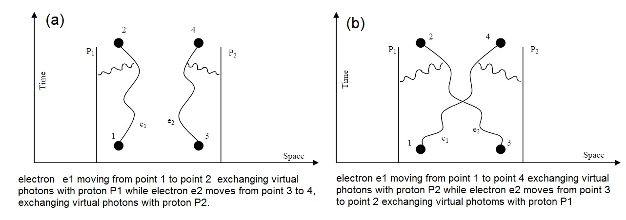
Fig 9. Illustrating bonding in the hydrogen molecule using Feynman diagram (from ref 205).
This is the essence of the MO theory for chemical bonding in the hydrogen molecule which is208“… based on the attractionsof two or more nuclei plus the averaged repulsions of the other electrons.” The additional influence of the extra nucleus on the atomic orbitals of the individual hydrogen atoms is treated as an interference effect and ends up as an overlap integral in MO-logy.
The Feynman diagram for the electromagnetic interaction via the electron-positron annihilation, with “electrons (and positrons) being represented by lines moving backward and forward in time, connecting by means of the absorption and emission of photons.”204, has been used205 for bonding in atoms and molecules as given above. As Anderson has cautioned204 the essential step in a derivation of Feynman diagrams is to turn on the interactions gradually and to assume that nothing discontinuous happens as we do in Fig 9. Anderson further cautions that bound states don’t form continuously, and therefore, there are serious difficulties in these treatments when bound states appear. Anderson’s example is the van der Waals’ short-range overlap repulsion due to the overlapping of electrons from one atom into bound orbitals on the other.
If the atom-bond transition itself is viewed8 as a discontinuous quantum phase transition, we may be faced with the same dilemma. In the scheme of Fig 9 the separate atom schemes of the Heitler-London theory is not used and is instead appropriate204 for the Hund-Mulliken MO scheme. In the Heitler-London-based VB theory a spin-dependent exchange interaction is calculated as an Heisenberg exchange integral. When such interactions involve localized electrons that are essentially bound states that are atomic in character, the Feynman diagram scheme is not applicable according to Anerson204. This could be the crux of the problem. The atom-bond transition is discontinuous and its description can be considered to be complete only when new particle or quasiparticle states are included.
One argues that the Feynman (or Feynman-like) diagrams are always necessary and valid when electromagnetic interactions are involved or when quantum field theoretical calculations are required for describing any interaction between elementary particles such as electrons, phonons, bosons that have their own free quantum fields. One only has to find the conditions for which the diagrams are applicable. We conjecture therefore that objections about bound states and Feynman diagrams may not arise when we examine the atom-bond transition at a m = 0 zero-chemical potential state. In this state, any interaction that takes a local m out of the stationary state is countered by forming an appropriately new state (particle or quasiparticle) that restore the system back to the m = 0 state. This it does by the emission or absorption of photons. A m = 0 system is a system in which the chemical potential, viewed as one in which there is no change in number with distance throughout the system for a given potential. Bader has stressed that “ … all systems are open systems that experience varying degrees of interaction through their shared zero-flux surfaces” such that Schwinger’s “… principle of stationary action for a proper open system is simply a generalization of quantum mechanics that applies to all physical systems.”
It seems to this author, trained strictly as a bench chemist, that there must be a stage in one’s efforts in understanding one’s chemistry when one must foray into applying Feynman-like diagrams to the world of various interactions¾bonded or non-bonded¾leading to various aspects of molecular structure, if for no other reason than to know how a gnarled untutored chemist interprets Feynman’s diagrams to suit his craft. It could even be useful, as we think we will show later, in finding universal geometrical aspects of bonding that is independent of the strength of the interaction,
Fortunately (or un-), thanks to the internet216-220, help is available. Feynman’s diagrams for elementary particle interactions come in the domain of quantum field theory where each particle has its own quantum field and each interaction is treated as a perturbation. The Feynman diagrams not only deal with light elementary particles such as electrons, positrons and quarks, but also with heavier particles such as “… messy balls of quarks, gluons, photons, virtual particles, elephant-antielephant pairs …” (from ref 216). The analogy of elephant-antielephant collision is not intended to be a doomsday collision with tremendous release of energy because of the heavy mass, but rather it is only meant to illustrate the possibility that there could be ways to examine interactions between heavy atoms that only involves the exchange of limited number of virtual photons in the process of forming, say, a chemical bond.
What follows is a mix of statements about Feynman’s diagrams from learned authors and attempts to take the first few steps towards understanding the chemical bond between atoms in general, avoiding as far as possible temptations of cutting and pasting. In doing so we end up with a diagrammatic variation where we do not need to conserve momentum or energy. Instead, we require just conserve the m = 0 condition for the chemical potential.
We have borrowed standard examples for Feynman’s diagrams for various interactions. In this notation an electron moves forward in time from left to right (Fig 10a) while a positron, which we have written as h+ instead of e+ to be consistent with our earlier usage and hopefully without dire theoretical consequences, moves in time from right to left; and the wiggly line is a photon that could be absorbed or emitted for the purpose of conserving momentum/energy. Given enough energy, the photon may produce heavier mass objects such as a muon-antimuon pair (Fig 10b).
In the world of chemistry it will not be wise to think in terms of matter-antimatter collision for understanding molecular structure or even normal chemical reactions. Yet, we have used11 the virtual photon of Fig 10a as a vacuum polarization for defining atomic sizes in a new way, remembering that in Feynman diagrams, internal lines, such as those in fig 10a, represent virtual particles that cannot be observed directly. We find such sizes to be useful, and Feynman-like diagrams could be considered seriously as symbolic representation of the ways that a particular structure may finally be formed by integrating allowed individual atom-atom interactions for every path.
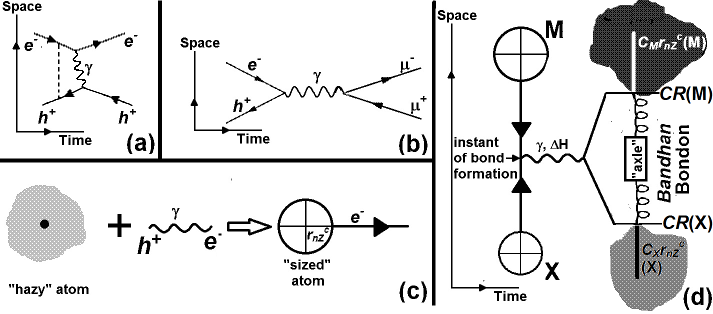
Fig 10.(a) Feynman diagram illustrating exchange of a photon (γ) between an electrons (e–) and a positron (h+). (b) Feynman diagram demonstrating annihilation of an electron (e–) and a positron (h+) into a photon (γ) that produces a muon (μ–) and anti-muon(μ+) pair later. (c) Defining the size, rnZc, of an “hazy” atom of atomic number, Z,by interaction with a virtual photon represented by an electron-positron (e–h+) pair; the atom is then represented by a virtual composite particle,Ũ where Å is a composite positively charged particle of Z electron and a virtual positron, h+, and ¨is a virtual electron. (d) Instant of bond-forming interaction between composite pariclesŨ(M) and Ũ(X) (rnZc(M) ³rnZc(X)) with the formation of new particles CR(M) and CR(X) that are composites of “hub” and “axle” components (see eqn 5) and has a bonding interaction between them; this interaction is here represented by the “axle” formed from bonding quasi-particles, which we name as “bondons”(in the Indian sub-continent this word is more easily recognized by the very romantic Sanskrit word, bandhan). Once the bond is formed the “hub” sizes, CMrnZc(M) and CXrnZc(X) are defined only in the direction of bonding for the given interaction, while the rest of the atom remains “hazy” in the absence of other interactions.
In the absence of any interaction our spatial concept of an atom does not assign it sharp boundaries. In this sense we may visualize the atom as rather “hazy” as to the left of Fig 10c. We avoid the use of the term “fuzzy” as it has been used in another context213, 214. Our contention that the size of an atom is defined only in the context of an interaction is sought to be illustrated in Fig 10c. More specifically, it is fixed by the positron-end, or h+-end, of the virtual photon Further, it has to be emphasized, that the size, which we have called rnZcwhich , is necessarily defined11 in the direction of maximum interaction for a given interaction field, and is therefore a one-dimensional size. It is the interaction of the valence electrons and inner-shell electrons with h+that “fixes and formulates” rnZc. This size is determined11 only for an energy-minimized stationary state and is consistent with a m = 0 condition for the chemical potential, which is the condition for obtaining inter-atomic distances in molecules. As such, the size rnZc is the starting size for all interactions and is scaled differently for different interactions (see, for example, Table 1) determining different inter-atomic distances. This isotropy in starting sizes is reflected in the symbol, Å, that we use in Fig 10c.
One assumes that the virtual positron annihilates an electron of the atom with atomic number, Z, so that one is left with a quasi-proton-like heavy nucleus, Å, with a positive charge and (Z-1) extra-nuclear electrons. The nucleus Å is left (“sprawling on a pin”) attached to an electron, e–,so that the Åe– composite is like a hydrogen atom.
We show in Fig 10d the first step in Feynman-like diagrams for obtaining inter-atomic distances. We actually focus on the bonding valence electrons. The two interacting atoms, say M and X (rnZc(M) ³rnZc(X)), move forward in time, with the bonding valence electrons converging at some point in space, determined by, say, the appropriate reaction cross section. At an “instant” (finite time) of bond-forming reaction, we assume that the valence electrons of the two interacting atoms, Å(M)-e– and Å(X)-e–, move in opposite directions (left of Fig 10d). Reaction is completed with liberation of energy (g, DH) to form new chemical species, CR(M) and CR(X), which are bonded by the “axle”. The sizes CR(M) and CR(X) have “hub” (Å) and “axle” components the values of which are fixed in space-time once the M-X bond is formed. The trajectory of CR(M) and CR(X) in space-time is nebulous in Fig 10dand the arrowless trajectory really should indicate that the overall charge neutrality is maintained.
The “axle” may be considered to be the essential part of a bonding between particles. The quasiparticles (see discussions around eqns 10 and 11 and refs 8 and 16) contributing to the “axle” size could be of the type shown in Table 1. In the diagram in Fig 10d, we have indicated the “hub” sizes CMrnZc(M) and CXrnZc(X) by straight lines (white and black, respectively) in the direction of the bond and in this way contributes to the M-X bond length. In directions other than the bonding interaction, the size of the atoms would remain hazy unless it is fixed and formulated by another interaction from another direction. We have called these bonding quasiparticles as “bondons”* and the bonding interaction is indicated by a looped line as used for gluons in Feynman diagrams. We imagine that there could be an analogy with the word “gluons” of particle physics if only because attachment is indicated by a glue and not because of the colour or charge of the gluon. The
—-
* We imagine the word “bondons” to be rooted in the very friendly Sanskrit word, “bandhan”. It means bonding of the non-repressive friendly kind¾bandhu means friend. There is a song from an old Hindi film “Rajnigandha” which has a newly married girl starting her married life and wondering about her bandhan which could mean bonding in an attachment sense. There is so much happiness in this bandhan,she sings. In the context of the chemical bond one could relate this happiness to a zero-chemical-potential state when the atoms in a molecule are in its comfortable quasi-free state with attractive and repulsive forces balancing each other; all the bondage is felt when the atoms are sought to be taken apart.
“bondons” are most-likely to be singlets and could correspond in some way to Lewis’ electron pairs for bonding. In this case, one may ignoramusly venture, to relate “bondons” to, if at all, the colourless spin-singlet gluons used to describe the strong force between hadrons such as protons and neutrons.The bondons are expected to have a real existence in the chemical bond of the hydrogen molecule.
It is immediately apparent from our description that there is no straightforward analogy with the molecular orbital or Heitler-London theory since they do not recognize the atom-bond transition as a quantum phase transition. Such a transition accommodates separate domains that define “hub” and “axle” sizes. Such sizes play a crucial direct-space role in determining molecular structure without really requiring a global energy minimization scheme.
An important feature in Table 1 that gives values of CPand DPis that no P-specific interaction-energy parameter has been used for obtaining the various sizes. The sizes CRPare thus obtained for a state which is free of all interaction potentials. This is the universal zero chemical potential, muniv = 0, state that is consistent with an energy minimized state that can even be local. Earlier, Politzer has noted221 that the electrostatic potential for an atom can be extended to molecules by summing over all constituent atoms. When this is done the expression for the molecular electrostatic principle contains only atom-like quantities without any cross terms. Politzer then went on to show that this implies that the chemical potential m = 0 condition is a good approximation and that the approximation becomes more accurate as the size of the molecule increases.
Chemical Potential of a Stationary State; Universal Value, muniv = 0.
It is commonly accepted that one requires an universal Thomas-Fermi-Dirac237, 238 value of the chemical potential for the stationary state, muniv = constant ¹ 0, for molecules or other phases condensed from atoms. Such a conclusion follows immediately from Sanderson’s principle239, 240 for the equalization of electronegativity and is primarily based on an interpretation of Teller’s theorem which states that a change of state cannot take place when m = 0. This condition usually follows235 from the condition that the maximum energy, EF(r) of an individual electron in an atom must be zero in order to prevent the electron from escaping to infinity. This requires EF(r) = pF2/2m + V(r)= 0 such that the kinetic energy is equal and opposite to the effective potential at r unless r ®¥, in this interpretation. The m = 0 condition is valid as long as there are repulsive and attractive forces that cancel each other.There has been, at the same time, a reluctance in acceptingthe Thomas-Fermi, m = 0, condition241, 242, 235applicable to free atoms themselves simply because such a condition seemingly precludes243(“The main failure of the TF model, its inability to allow atoms to combine to form a molecule” at m = 0) the condition for reaction which necessarily involves a change of energy.
There has been a reluctance to accept a Thomas-Fermi-like muniv = 0 condition for the chemical potential condition for the stationary state, mainly because of Teller’s theorem35 or 243, 236 by which the Thomas Fermi molecule (containing more than one nucleus) is unstable relative to separation to atoms primarily due to repulsion between nuclei (see later). “Teller’s proof is a very clever one, involving a fair amount of chitchat but almost no mathematics, but the proof is not without weakness” (from ref 235). There has been, at the same time, several learned discourses consistent with a condition, muniv = 0, for the stationary state221, 241, 245, 246 of an atom or a molecule. One could adopt the view that any perturbation that disturbs the m = 0 condition for the stationary state is a reaction-initiation condition at the instant of a m¹ 0 condition. When the stationary state is reached the m = 0 condition applicable to a free atom is restored. It is for this condition that one could use atomic sizes that contribute to inter-atomic separation in a molecule and which satisfy the muniv = 0 condition8.
There is not much disagreement regarding the existence of a constant universal value of the chemical potential being a constant, muniv = constant. This follows for example electronegativity equalization principle of Sanderson239,240. The requirement of m¹ 0 also appears in the Weiszacker and Dirac-exchange correction to the Thomas-Fermi value238. It has been commented that a constant value of the chemical potential has little usefulness as far as understanding the ground state is concerned245. The constant chemical potential term may be arbitrarily chosen for different energy scales and it would be important to find the universal scale. On the other hand the muniv = 0 condition is a more restrictive condition. A m = 0 condition for the stationary state requires that the rate of change in the energy with respect to any perturbing parameter in the stationary, energy minimized, density optimized, state is zero. This condition does not depend on the energy scale. The distinct advantage on adopting the m = 0 condition for the stationary state is that atomic parameters (such as a size) obtained under these conditions would be valid and transferable from atom to molecule for an energy-minimized condition!
One of the early alternatives to complex wave mechanical approaches is the Hellmann-Feynman theorem. This is a classical electrostatic approach in which one examines forces acting on a nucleus due to other nuclei and the density of electrons distributed around the nucleus. The total energy of a system is then related to the values of the electrostatic potential felt at the positions of the nuclei The Hellman-Feynmann theorem252, 253, 203 is a mathematical statement that describes the role of charge density in chemical bonding¾there is a set of nuclei held together by electrostatic attraction to the charge density. This theorem relates the total energy of an atom or molecule to the electrostatic potential that is created at any nucleus by the electrons and remaining nuclei in a molecule. For an exact eigenfunction y of an Hamiltonian H(l) with an eigenvalue E(l), the Hellmann-Feynman theorem is
¶E/¶l = áy½¶H/¶l½yñ/áy½yñ (45)
wherel is any parameter in the Hamiltonian, H. It is known from the “electrostatic Hellmann-Feynmann theorem” that the force acting on any nucleus in a system of nuclei and electrons can be “interpreted solely in terms of classical electrostatics” even if the actual charge density may be required to be obtained by a quantum mechanical procedure203. Such a force on a particle is necessarily a resultant of the forces due to the other electrons and nuclei. For an energy-minimized stationary state the resultant force acting on any particle (nucleus or electron) vanishes so that an equilibrium molecular geometry may be obtained from this condition. The force and energy pictures are therefore equivalent as far as stationary properties are concerned. It is interesting that such a balance of forces prompted Bragg285 to find a parallel with engineering structures: “We may compare this case of crystal equilibrium to the engineering problem of calculating the stresses to which the member of a a girder system are subjected. … We can try and explain the properties of the crystal as a whole by making certain simple assumptions about the forces between the atoms.” This mechanical approach is reminiscent of Buckminster Fuller’s more endearing structural engineering tensional integrity (tensegrity) concept287, 288 based on balance between tensile and compressional elements in tensegrity structures such that compressional aspects are reduced and there is no collapse. We will use this concept later to discuss the role of molecular tensegrity60 in the way 1,3- non-bonded distances as a balance between repulsive 1,3- forces and attractive 1,2- distances as gauged purely by atomic sizes.
An important additional advantage in terms of such Hellmann-Feynman force considerations is that the single particle picture becomes valid especially when the electron and nuclear coordinates are independent of each other (as, say, within the adiabatic approximation). Politzer and coworkers221,244 have extensively studied the properties of atoms and molecules as expressed by the electrostatic potential the significance of which goes beyond the interaction energies. The important point is that the electrostatic potential is linked rigorously to r(r) by Poisson’s equation, which in turn is related through the Hohenberg Kohn theorem to the system’s properties.
In order to find and exploit such a condition from first principle ab initio calculations it is generally assumed that the stationary state properties of an atom or molecule, requires a knowledge of the exact single particle density. A difficulty in this approach, therefore, is that the applicability of the Hellmann-Feynman theorem is very sensitive to the accuracy of the wave function.
Variable Inter-atomic Distances

Fig 11. Two different views of a 1D potential energy diagram. Full line: normal view point; dashed line: energy minima located at different distances (adapted from Parkin, ref 223)
The traditional view of a single minimum on the ground state potential energy surface (full line Fig 11) as a function of separation between the two bonding atoms, is to allow only a single distance, which is the bond length between atoms. The first paper to highlight in its title the possibility of bond-stretch isomerism¾“… a novel type of isomerism in which two or more stable conformations of a molecule related to each other by a simple bond stretching differ in their electronic configurations…” is due to Stohrer and Hoffmann225, Bond–stretch isomerism has been described by the existence of separate energy minima on a global potential energy curve between the atoms with a significant barrier between the minima. This “as counterintuitive as it is fascinating”223 possibility is sketched in Fig 11 by dashed lines.
Ideally, one requires a case where bond length changes are not related to changes in spin-state, valence state, disorder, ligand deformation and so on. The status of this phenomenon is still a little ambiguous ranging from “not credible”227 “fact not fiction”228. The way a particular collection of particles in non-interacting atoms (at high temperatures) approaches its stationary point configuration in a chemical bond (Fig 11) may be represented as a 1D funnel in energy landscape perspectives. The high-energy, high-temperature state could encounter various metastable states en route to the ground-state configuration for the given ambience as shown in Fig 11. The local minima at intermediate energies correspond to possible M-X distances.
In the way Fig 11 is drawn, every local minimum would correspond to a m = 0 condition (eqn 1) for the given environment. There are various ways to reach the m = 0 state. We assume from eqn 1 that any point in the trajectory marked by a minimum in energy is a stationary state. This m = 0 condition is applicable to any stationary point and not only to that of a global minimum. In the “hub-and-axle” model that we have adopted such changes can be accommodated by different “hub” and “axle” sizes, with the condition that such sizes separately satisfy the m = 0 condition. These are first order changes and are to be distinguished from changes in equilibrium distances that are caused, say, by changes in the dielectric properties of the medium, or due to small second order differences due to changes in environment arising from a recurring principle of causality. Such small changes are of interest, for example, to pharamaceutical industry223, 230, 231.
In what follows we examine the way the values of CM, CX, DM and DX may have different values, even when rnZc is not changed (valence state, spin-state is not changed). What one requires is a description in which the existence of different minima on the potential energy contour is to be expected to be of first order. One major aspect that we focus on is the way the problem of spin conservation can be handled in atom-bond transition when two doublet valence electrons are paired to form singlets in the chemical bond. One way to examine this problem is at the “instant” of bond formation sketched in Fig 10d. In the way the “instant” is visualized¾arrows in opposite directions¾space-time, there is an implication that the interaction involves opposite charges or opposing magnetic moments due to opposite directions of electron flow. This would form the basis for the two different types of bond-formation¾“charge-transfer” (referred to hereafter as CT) or “neutral” (Nn)¾that we have listed in Table 1. As we shall see/use later there could be contributions of CM, CX, DM and DX to “axle” or “hub” sizes that are different from those listed in Table 1. We suspect that our arguments are robust (because of the way we account for inter-atomic distances later) and that they have not been used earlier because the atom-bond transition has not been examined at the m = 0 condition,
Spin Conservation at the Atom-Bond Transition.
Many important physico-chemical processes involve the conversion of a pair of doublet electrons to singlet pairs in which the spin is not conserved. The simplest of these non-conserving spin processes is the atom-bond transition (ABT) when doublet valence electrons on two different atoms form a singlet bonding pair of electrons in the chemical bond. Such transitions may be viewed as a quantum phase transition with a crossing of a phase boundary15. It is difficult to follow by a one-to-one mapping the change from the two-doublet system to a system with a singlet state. One is therefore not likely to obtain information about inter-atomic bonding processes by a renormalizaton of our understanding of intra-atomic properties. Yet, the specific role of the spin statistics or probabilities must manifest itself in some way that determines, for instance, chemical bond lengths after an ABT.
An area where this problem is recognized and pursued vigorously is that of the singlet-triplet transitions in the chemistry of biradicals. Conventional treatments263, 264 of spin-chemical effects are complicated because of considerations of various processes such as spin dynamics, kinetics of spin-selective reactions, spin relaxation and molecular motions.
Spin-conservation rules are important at every step where spin-conserving decisions are required during the atom-bond transition. For example, two doublets would react to form spin-forbidden singlet products if there is some probability that the two electrons are aligned anti-parallel at the instant that the bonding S = 0 singlet state is formed. One requires the probability for finding this instant. An additional complication appears when we consider the “hub” electrons wandering in and out of the “axle” regions and vice-versa. The bonding or “axle” region has spin-constraints (such as being aligned antiparallel) on the bonding pair of electrons while there need be no such constraint between the electrons in the “hub” of an atom that is imposed by the bonding electrons once the m = 0 stationary state is reached. However, because of the indistinguishable nature of electrons the system requires some adjustments such that such different constraints on the spin in the “hub” and “axle” are absent once the bond is formed and all particles are at muniv = 0. We show below, that the constants CP is a measure of the way the “core” atomic sizes have to be scaled so that total spin is conserved at every instant of an exchange of indistinguishable electrons between “hub” and “axle” regions.
The way this spin-pairing is handled in conventional wave-function based quantum-chemical approaches is simply to use the Pauli Exclusion Principle and antisymmetrising the spatial and spin part of the wave functions assuming that the total spin is conserved. In this approach the eigenfunctions of the Hamiltonian, H, become also eigenfunctions of the total spin with common eigenstates of H, S2, and Sz. The computational-time problems rise in finding some quantitative estimate of the probability for this instant of reaction using conventional quantum chemical methods when every perturbation requires a renormalization of the wave function or density functional at a non-zero chemical potential. This is necessary to drive the reaction to completion so as to reach a zero chemical potential of an energy-minimized state.
In order to be more specific we may first consider a general perspective on the Atom-Bond Transition (ABT). The bond-forming reaction between two sites M and X is schematically given in eqns 5a – 5d. Neutral quasi hydrogen-like atoms of atomic number Z are denoted as Ũ, where Å represents a “pseudo core” with (Z – 1) extra-nuclear electrons. The pseudo “core”, Å, has a neutral (doublet) spin ½ valence electron, ¨. Bond formation is initiated at that instant at which the spins of the two valence electrons are aligned anti-parallel to each other to form a singlet state in a molecular biradical (RHS of eqn 46a)
{ŨM}S=1/2 + {ŨX}S=1/2® {(ÅM)S=1/2 + (ůX)S=-1/2}SS =0 (46a)
The singlet biradical state of eqn 5a is favorably poised to form a spin-less bonded state when a spin-conserving transition is allowed and a “neutral” chemical bond (eqn 46b) is formed.
{(ÅM)S=1/2 + (ůX)S=-1/2}SS =0 ® {[ůÅ]MX}S = 0 (46b)
The way the “neutral” bond is formed is outside the scope of this article. Further evolution of the chemical bonding involves “charge-transfer”. We visualize the formation of charge-transfer to be preceded by the absorption of an electron-hole pair, [e–h+] as in eqn 46c followed by the formation of the “charge-transfer” bond as in eqn 46d.
{[ůÅ] MX }S=0 + [e–h+] « {[ÅM(·h+)]+ + [(e–·)Å]–X }S=0 (46c)
{[ÅM(·h+)]+ + [(e–·)Å]–X}S=0® {ÅMð+(··)–ÅX }S=0 (46d)
The particles (·h+) and (·e–) of eqn 46c are the bonding quasiparticles24 that exist only in the “charge-transfer” bond (eqn 46d). They have been proposed to account for the “ordinary” bond length of the hydrogen molecule. The charge-transfer (CT) bonded state is the RHS of eqn 46d. The (·h+) and (·e–) particles proposed in eqn 46c for the hydrogen molecule have a parallel with Bogoliubov quasiparticles25 which come in pairs of eigenvalues that are exactly symmetrical with respect to each other about the chemical potential. The sizes, D0+ and D0–,of such quasiparticles (Table 1) have been obtained by using such a symmetry about a universal condition, muniv = 0, for the chemical potential.
Our interest in this communication is to find the probability, p¯, of forming the singlet state in the RHS of eqn 46a from the two doublet states on the LHS of eqn 46a. We also seek to find the probability, p··, of forming the charged state [··]– from the two doublets after the spins have been annihilated. We find it sufficient to obtain information about these probabilities using a simple interpretation of the Buffon needle problem.
The Buffon Needle Problem.
The Buffon’s Needle problem, the first in what is now known generally as Monte Carlo methods, is a branch of geometric probability265. 266 or integral geometry that is concerned purely with probabilities associated with finding a geometrical configuration. To the best of this author’s knowledge, the first attempt to apply the Buffon needle problem to the probability of finding a given orientation of the spin of an electron has been made16or20 in the context of the insulator-metal transition.
In the classic Buffon needle case one commences with parallel equidistant lines on a plane spaced a distance, d,apart. One throws a needle of length, l, randomly on this plane such that the location of the centre of the needle and its orientations are uniformly distributed. When l£d, the probability, p½, that the needle will cross one the lines is given by
p½ = 2l/pd (47)
In the simple Buffon problem on simply counts the number, N’, of times the needle crosses the line for a large number of throws, N. The ratio N’/N is expected to be given as 2/p when l = d. Implicit in the usual Buffon needle argument, is that the needle itself is treated as a direction-less straight cylindrical thin rod (or line) although a needle itself, with an eye and a point, has really a direction. Once a particular orientation is required of the Buffon needle one would expect, assuming a double-valuedness (“… due to a peculiar classically not describable … quantum theoretical properties of the valence electron …”, Pauli 1924) the probability p, is the probability of finding an orientation in a particular given direction. One expects
p = p½/2 = 1/p (48)
From these simple considerations of p½ and p one may now arrive at probabilities of spin-alignments for the various states in eqns 46 between two sites assuming that the starting probability, p1/2,1/2 of two doublets (LHS of eqn 46a) is unity.
The probability of finding an “up” spin orientation would be the same as finding the “down” spin orientation, or p(M) = p¯(M).The probability of finding two spins aligned in a given direction relative to each other will depend on the product of the probability, p(M), of finding an orientation of the spin of the concerned bonding valence electron at the site M and simultaneously finding the required orientation, say p¯(X). The total probability, pM,X, of finding the spins with a given orientation, say, antiparallel with respect to each other, is given by pM,X = p(M)p¯(X).Once one requires a given spin orientation, say, at the instant of a singlet, ¯, formation the probability of finding such an orientation would be from eqn 48
p¯ = (p)2 = 1/p2 = 0.101 (49)
By this argument, given two fixed orientations, the probability for finding the two orientations starting from two randomly oriented electron spin doublets would be the same, e.g., p¯ = p = 1/p2.
The probability, p¯, for finding a singlet state is expected to different from the probability, p··, for finding a spin-less charged state. In the case of the spin-less charged [··]– state (RHS of eqn 46d) we consider spin-less rods, ½, since the orientations of the individual spins are degenerate in the charged state. The probability p½½(={(p½i)(p½j)}) of having a correlated orientation of spins on electrons i and j, in a [··]– charge is (p½)2 = 4/p2 from eqn 47. The probability, p··, of spin conservation of the valence electrons on going from two doublet states (LHS of eqn 46a) to the charged state [··]– (RHS of eqn 46d) through singlet spin states, [¯] (RHS of eqn 46a), is
p··=2{(p¯)´p½½)}= 2(1/p2)(4/p2) = 8/p4 ~ 0.082 (50)
after taking into account the degeneracy of the two spin configurations in the spin-less electron pairs of the chargon [··]–. From eqns 49 and 50, p¯>p··, which is consistent with the intuition that spin has to be annihilated in charge-less “spinons” before spin-less “chargons” are formed.
“Charge-Transfer” Bond Lengths.
In a chemical bond, the spins of the bonding electron pair are already paired to in the “charge-transfer” {ÅM+(··)ÅX–} (RHS of eqn 46d) so that spin-conservation probabilities, p¯ or p··, do not directly appear when considering dMX. They appear indirectly, however. We consider the spins on the electrons of the “pseudo core” atoms, ÅM and ÅX, to be decoupled from those in the spin-less bonding pair of electrons, (··)–. When this is done, the probability, pexch, for sustaining the spin-pairing in the bonding electron pair on exchange of electrons between the “pseudo cores” ÅM and ÅX and the bonding valence electron pair would be reduced from unity. Because electrons are indistinguishable, however, one requires compensating for pexch< 1. We propose that the volume of the atom has to be increased by 1/pexch, so as to sustain conservation of spin and maintain the condition for indistinguishable “pseudo core” as well as “bonding”electrons in an atom. The coefficients C+ and C– in Table 1 that define the “hub” size of the M and X atoms, respectively, may be seen as factors that are obtained from pexch-1.
The “instant” of initiation of bond formation as expressed in eqn 5a is the instant when individual valence electron spins on atom become annihilated as bond formation proceeds. When M is more electropositive than X, the instant of bond formation may be thought of as initiating the formation of M+ with a probability p¯ = 1/p2. In order to sustain the exchange of electrons between the “pseudo core” atoms ÅMand the bonding electron pairs one requires 1/pexch(M) = 1/(p¯) = p2. The size of the M atom, rnZc(M), then has to be increased by (1/pexch(M)1/3) = C+. We thus obtain C+ = p2/3 ~ 2.145. Similarly, from eqn 46 the values for C– would be given by C– =1/pexch(X) = 1/(p··)1/3 = p4/3/2» 2.300. This justifies the use of these values in earlier21-23 publications (Table 1).
Since the values of the charge-transfer coefficients C+ and C– depends on probabilities of orientation of a spin on the valence electron, it is necessary that the conditions of the ratio (eqn 22) of the residence time, tW, vis-a-vis the internal Larmor precession time, tLint, would play an important role in determining whether CT or Nn values should be used. As we have discussed earlier, the spin is well defined when tLint<tW.
tW / tLint= J/4t = Pt/4U. (22)
As the transfer integral increases for a fixed value of the correlation gap U, we have two limits (from Eq. 22)
- i) Pt /4U> 1. From Eq. (22) tLint<tW, such that the spin of the electron is well-defined by its internal Larmor period, tLint, for the time defining the charge at a site. The spin excitation gap is smaller than the bandwidth. The Mott-Hubbard criterion125 for metallization, Wb³ 2U is satisfied for z³ P/4 such that even z = 1 (as in a chemical bond) satisfies the Mott_Hubbard criterion for metallization.
- ii) Pt /4U< 1 J/t< P/4 and tLint>tWunder these conditions. The residence time of a charge-carrier at its site, tW (defined by t), is less than the J-dependentLarmor precession period, tLint. The direction and/or magnitude of the internal field, Hexc changes with every t-dependent transfer of the spin-less charge. The spin-excitation gap is larger than the bandwidth in such cases. An itinerant electron state in which there are sites with Pt/U < 1 (for same values of z)would have slower relaxation dynamics for spin as compared to charge. Because of this, such systems may behave as non-Fermi liquids.
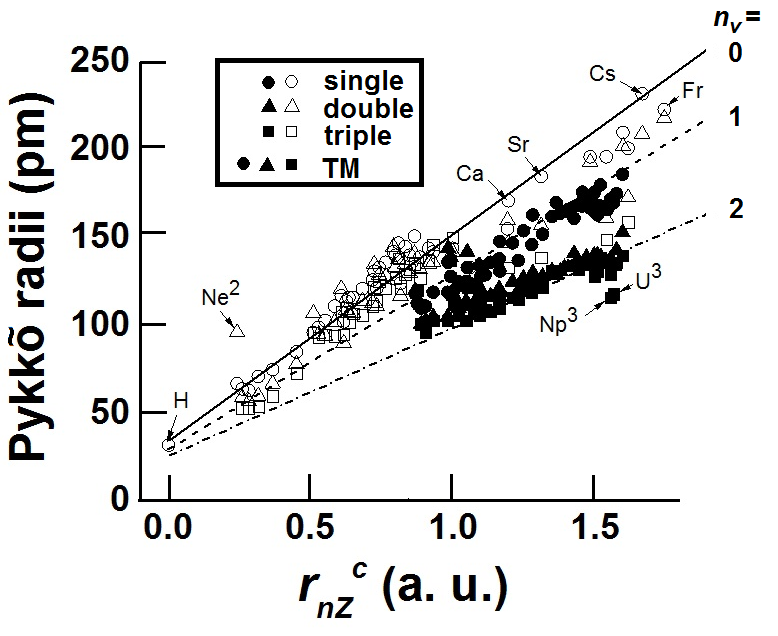
Non-Bonded Distances
The van der Waals’ interaction is usually between gas phase molecules where the separation between atoms is much larger than a van der Waals’ radiusrvdW. These sizes as defined by Pauling are obtained from non-bonded contact distances in molecular crystals between two chosen atoms which are already bonded to other atoms. These atoms are usually peripheral atoms of a molecule. The accepted refinement of Pauling’s radii are due to Bondi whose tabulated radii, rBondi, are found to be especially suitable for small organic molecules (Gavezzotti, A. J. Am. Chem. Soc. 1983, 105, 1983; Rowland, R. S.; Taylor, R. J. Phys. Chem. 1996, 100, 7384). Further, its values are usually considered to be uncertain when applied to atoms of metallic elements (S-Z. Hu,, Z-H Zhou and B. E. Robertson, Z. Kristallogr. 224 (2009) 375–383; M. Mantina, A. C. Chamberlin, R. Valero, C. J. Cramer, and D. G. Truhlar, J. Phys. Chem. A 2009, 113, 5806–5812). The theoretical foundation for the so-called van der Waals’ contact distances between atoms in solids is further constrained by the uncertainty of magnetoelectric influences which are likely to be strong (S. Y. Buhmann, H. Safari, H. T. Dung, and D. -G. Welsch, Optics and Spectroscopy, 2007, 103, 374–387).
The vdW interaction was first calculated in the non-retarded limit by London on the basis of perturbation theory, who found an attractive potential proportional to r–6, where r denotes the inter-atomic separation [1F. London, Z. Phys. 63, 245 (1930); Z. Phys. Chem. Abt. B 11, 222 (1930).]. The van der Waals (vdW) interaction of two neutral, unpolarized, but polarizable atoms is thought to arise from ground state fluctuations of the electron configuration of these atoms. For sufficiently small separations, its physical origin may be seen in the electrostatic Coulomb interaction of the atoms’ fluctuating dipole momentsdue to quantum ground state fluctuations.
As a first approximation we may consider the electrons in the valence shell of atoms A and B that are involved in the interaction is a spin-less electron pair [··] which, after a bond is formed, may be considered to be charge-less. Since an electron cannot be fractured, these interactions involve fluctuations in occupancy of single electrons. Thefluctuations must, at the instant of polarization, involve excitations of an integral number of electrons. Such interactions arise. The spin of the single electron could play an important part when conservation of spin is important.
We may consider these quantum fluctuations in van der Waals’ interactions, to be represented by the absorption of a vacuum-polarization represented by an electron-hole pair, [e–h+], as
[··]A + [··]B [e–h+] « [··e–]A + [··h+]B« [··, ¨]–A + [¨]+B (10a)
º [··, ]–A + [¯]+B« [··, ¯]–A + []+B (10b)
« [¨]+A + [··, ¨]–B«[··h+]A + [··e–]B (10c)
º [··]A + [··]B [e–h+] (10d)
The transition from the doublet, ¨, states of eqns 10a and 10c, RHS of eqn 10a to the spin-aligned states of eqn 10b would still depend on a spin-alignment probability, which we term as pvdW. One expects in the direction of interaction pvdW= (Kp··)p·· = K(p··)2 = K(8/p4)2. The term K is a term that addresses the degeneracy of the various states in the context of the dispersion interaction. It would seem that since the van derWaals’ interaction is through fluctuations in whole space, the term K is a probability factor that is valid in all dimensions. One expects K = 2.
One may use arguments similar to those used for obtaining C+ (or C–) from p¯ (or p··). These terms are obtained from considerations of the increase in volume required to sustain exchange of electrons between other parts of the atom despite a probability less than unity for p¯ or p··. However, the crucial difference in calculating the corresponding value of CvdW = K(p··)2/3 instead of (KpvdW)1/3. We thus obtain the ratio
CvdW/C–X = (1/{K(p··)1/3}=(p4/3/4) = C–/2 = 1.150
when K= 2.
One-electron non-localized wavefunctions (MOs) describes each electron in a molecule with a known geometry. Thus, each electron
has been assigned a one-electron function (an orbital), and
the repulsion between the electrons has only been treated
on the average.
The “size” of an atom is very important for its chemical
behavior. A possible measure of this is the expectation
value (mean value) (r) of the distance of the valence electrons
from the nucleus. Quantum-chemically calculated[301
values of (r) for s and p valence AOs are depicted in Figure
2.
First, it should be noted that (r)s and (r),, for the first row
differ little from one another (by ca. lo%), whereas for
higher rows the differences are more pronounced (20-
33% for the second row; 24-40% for the third and fourth
rows; and 36-55% for the fifth row).
Furthermore, we observe that árñp3/2/ and árñp1/2 differ
from each other by less than 2% for the first three rows, by
- 5% in the fourth row, and by as much as ca. 15% in the
fifth row. Within the framework of “ordinary” nonrelativistic
quantum mechanics, such as in conventional Hartree-
Fock calculations, there is no difference between p1/2 and p3/2, and the p level is sixfold degenerate (threefold orbital
degeneracy and a twofold spin degeneracy). The splitting
into a twofold degenerate p1/2 and a fourfold degenerate
p3/2 level is a relativistic effect which depends on so-called
spin-orbit coupling. In the fifth row, the two possible p
states differ from each other almost as much as the s and p
(the effect is even more marked in the orbital energies than
in the radii). This relativistic effect has major consequences
for the chemical behavior of the very heavy elements[
26-281
Gas-Phase Diatomic Compounds
The analysis of inter-atomic distance in gas-phase diatomic MX compounds is expected to be truly representative of the influence of core sizes on bonded inter-atomic distances as no effect due to non-bonded interactions involving other atoms is expected.We have shown in Fig 9 the plots of observed distance vs the calculated distances. At first glance, it would seem that most of the observed107M-X distances listed for gas-phase diatomic MX compounds, fall within that expected using “charge-transfer” “hub” and “axle” sizes and with nv£ 2. However, as discussed earlier20, there is a scope for the use of “neutral” sizes also, once eqn 37 is used to distinguish between “static” and “peripatetic” compounds.
distinction between “as indicated in Tables 1 and 2.
MX compounds which are considered to be “static” (do not satisfy eqn 37) usually have have “charge-transfer” “axle” sizes, DMX = 4aH/3m, with the main exceptions being the inter-halogen compounds which may be better fitted using “neutral” “axle” sizes. “Peripatetic” MX compounds (satisfying eqn 37) have “neutral” “hub” as well as “neutral” “axle” sizes. We have earlier calculated the electron number profile across the bond axis for some representative examples of gas-phase MX compoundbased on the density functional B3LYP calculations23.

Fig 9. Plots of observed106,107 M-X distances in gas-phase diatomic MX compounds vs the calculated single-bond (nv(M) = nv(X) = 0) charge-transfer distance, d00±. (a) for M-X compounds that do not satisfy eqn 37. (b) MX compounds that satisfy eqn 37. Dashed straight lines are meant as a guide to the eye for the correct fit. Straight lines meant as a guide to the eye for nv = 1 (“double bond”) and nv =2 (“triple bond”) are also shown.
The usual quantum chemical calculations consider the system as a whole and not its component parts. Indeed, the aim of Bader’s AIM (atom-in-molecule) approach, which uses the principle of the Schwinger stationary action, is to correctly estimate from a partitioning of the electron density, characteristic chemical concepts such as the size of the atom, and the chemical bond especially. In our analyses of isolated M-X bond in gas-phase diatomic MX compounds we have calculated the electron number profiles, EN(r), using the quasi-empirical but purportedly ab initio B3LYP DFT method. The calculated electron number profile, EN(r), corresponds well to the calculated inter-atomic distance using CMCXDMX where CMrnZc(M) and CXrnZc(X), give the “hub” sizes of the M and X atoms, respectively, DMX is the “axle” size. Of interest is the feature that one may assign a dimension (the “axle” size) to the two bonding valence electrons along the bond axis. On the other hand EN(r) has contributions to the bond distance from the “hub” sizes of (ZM/2 – 1), and (ZX/2 -1) from the two bonding M and X atoms, respectively, which are each one electron short compared to that expected from their atomic number ZM and ZX , respectively.
This important aspect is a reminder of the assumption that the core sizes rnZc have been obtained in the presence of an interaction represented by a virtual charged photon, [h+e–]. The h+ interacts with nval valence electrons to define the size rnZc so that rnZc is ultimately the size of ZM,Xelectrons of the atoms M or X and a hole, h+, of the virtual photon. There is therefore only (ZM,X -1) electron in the “hub” region defined by CM,XrnZc(M,X). The valence electrons in “axle” region therefore may be thought to represent the electrons of virtual photon [h+e–]. It is therefore some surprise that the DFT B3LYP method should so neatly give the partitioning between “hub” and “axle” regions without specifically building in such an assumption into its starting premises. It is clear that some of the results of different calculations should appear similar since the calculations are aimed at obtaining an energy-minimized state from considerations of coulomb interactions which are common between them. On the other hand, it is not clear that spatial distribution of density of particles obtained from these calculations represent at best a time-averaged distribution.
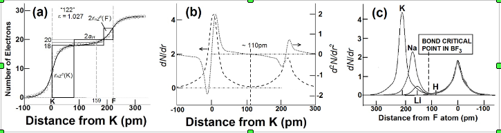
Fig 10. (a) Plots of electron number, EN(r), along the bond axis as obtained from B3LYP calculations (ref 23) on KF showing the matching to CKCFDKF= 1.2.2. As per the calculation EN(r) = 19 at ~ 150 pm from the nucleus of K. (b) Plots of 1st (dashes) and 2nd derivative (dots) of EN(r)with respect to r of KF. (c) Plots of 1st derivative of EN(r) with respect to r for KF, NaF, LiF and HF.
col(d)-col(G1)
A typical result of a B3LYP calculation23 of the electron number profile across the bond axis is shown m Fig 10a for KF which satisfies the “peripatetic” condition of eqn 37.. It is seen that “neutral” values of CKCFDKF= 1,2,2 fit the observed distance well (dKF122(cal) = 211 pm, dKF(obs) = 217 pm; eKF ~ 1.027 from eqn 7). It is seen that EN(r) = 19 = ZK about 160 pm from the K atom suggesting that the atomic limit of K is about 160 pm from its nucleus in one criterion. The electron density along the bond axis is plotted as dN/dr in Fig 10b (dashed line). The second derivative of EN(r), d2N/dr2, would correspond a 1D equivalent of Bader’s Laplacian of the electron density. Accordingly, the point where d2N/dr2 = 0 would correspond to Bader’s definition of the bond critical point, or the size of the atomic basinof K in the bonding direction. This distance is nearly 115 pm from K and does not correspond to any size¾”hub” and/or “axle”¾that can be related to parameters of our model.
We have shown in Fig 10c the plot of the 1st derivative of EN(r) with respect to distance from the F atom (we show in parentheses the dMXCMCXDMXe(MX)used in the calculations) for HF (dFH1-4/31.01), LiF (dLiF1,2,4/31.02), NaF (dNaF1,1.5,21.02)and KF (dKF2121.03).The envelope of dN/dr around the F atom is fairly superimposable indicating that the environment around the F atom does not change despite changes in CF as well as DMF.It is also seen that, except for HF,the position of the minimum in dN/dr in all these compounds is close to 105 pm. This minimum would also correspond to d2N/dr2 = 0 or to the intersection of Bader’s zero-flux surface with the bond axis or the bond critical point. At this point the Laplacian, Ñr(r) = 0and defines the inter-atomic interface of the bond. As already mentioned above, this bond critical point point does not correspond to the number of electrons given, say, by ZF or ZM. We find that the distance of the bond critical point from the fluorine atom in BF3 as extrapolated from (Fig 2 of ref 200) is also close to 105 pm. Thus although size of the atomic basins in a Bader-like AIM approach does not change with its bonding M atom thereby trult representin the AIM, the EN(r), profile correctly reflects the changes in the CMCFDMF values without necessarily correlating with the bond critical point parameters.
It is perhaps necessary at this stage to briefly distinguish between the philosophies of Bader’s AIM approach and the approach adopted by us. As stated by Bader, one treats an atom as part of an open system that is subject to changes in number/charge and position/momentum in the system with time. In the non-relativistic limit, the motion of a particle moving in a potential V(r, t) where rand t areindependent variables is described by a Lagrangian.
Schwinger approached the problem by changing the initial and final time infinitesimally. Schwinger’s principle of stationary action for a given dynamical system states that changes associated with the two end points in time define the changes in the action integral operator. The atom in an open system is then defined by the evolution in time of its spatial boundary202. Bader emphasized the point that for a zero-flux boundary condition the action integral is of the same form as an isolated system. Bader then went on to define the boundary of an atomic basin in terms of a three-dimensional space around its nucleus without invoking a time derivative that forms the basis of Schwinger’s action principle. What is not clear is the way the interaction between two atoms, separated by a bond critical point, is related to the bond critical point.
In the Hamiltonian approach of Heisenberg, Schrödinger, Dirac, a given interaction field is treated as a collection of harmonic oscillators, with the electron system being always in its ground state. As pointed out by Feynman201 the oscillator can be eliminated and replaced by a direct interaction. One would be interested in the way the space-time path is changed between the time the interaction is switched on and the time the system comes to rest subsequently. If A is an action functional that describes the character of a space-time path and assigns a number to each possible mechanical path, q1(σ), q2(σ) . . . qN(σ), the N equations of motion according to the principle of least action are given by,δA/δq1(t) = 0, δA/δq2(t) = 0, . . , δA/δqN(t) = 0.
Once the state of least action has been obtained, the electrostatic Hellmann-Feynman theorem states203 that classical electrostatics may be used to describe a system of charged particles such as nuclei and electrons. The equilibrium molecular geometry is thus the configuration in which in which the net force on any charged particle vanishes. This also corresponds to the energy minimum. The equivalence of force and energy minimum is a matter of principle even if, for calculation purposes, this equivalence would depend on the accuracy of the wave function203.For energy functionals, E,stable stationary states are associated with local minima associated typically with a local ¶E/¶ri = 0 as well as a global Si¶E /¶ri = 0 (eqn 1). This is the condition that the chemical potential, m, satisfies the universal condition muniv = 0.
Our “hub-and-axle” model, reinforced by DFT calculations asserts, that the principle of least action requires that the muniv = 0 condition is obeyed separately for the “hub” and “axle” components. The “axle” incorporates the interaction between the atoms. In the case of the “charge-transfer” bonding the “axle” size, such as that for the hydrogen molecule in eqn 13, involves bonding quasiparticles, (e0h+) and (e0e–) arising from interaction with a charged virtual photon [h+e–]. In the case of “neutral” “axle” sizes we envisage the participation of “neutral” spin-½ hydrogen-atom-like particles which we write asÅwhich condenses to form spin-singlet ůŠ“neutral” bonds through the magnetic equivalent discussed in the section on the “Magnetic Bohr Model”.
The important point is that the “axle” as well as the “hub” sizes is built into the “atom-bond” transition in our model once one interaction with vacuum polarizations are included.From the way the size rnZc is obtained11, the size of the “hub” includes one virtual hole of the virtual photon, [h+e–],and Zelectrons of the atom with atomic number, Z,or virtually (if not effectively) (Z – 1) electrons. The “axle” size is then obtained from interactions involving the virtual electron of [h+e–]. Such interactions would make the “axle” an equivalent of an harmonic oscillator. It is not possible to obtain this informationon inter-atomic interactions simply by a renormalization of ourunderstanding of intra-atomic processes.The number of electrons in the “hub” and the “axle” regions is thus determined by the interaction involving [h+e–].It is curious that we are able to reproduce features of Bader’s AIM approach as well as the “hub” and “axle” sizes of our approach using “real” electron number profiles, EN(r), obtained bythe DFT B3LYP method which does not specifically break up the electron system into core and valence regions the way we have, using atomic sizes that are defined by interactions with vacuum polarizations. It is nevertheless satisfying that the computed EN(r) fits “hub-and-axle” domainsinto the .
-like bond critical pont BF(dBF1,2,4/31.04). BF3(dBF2,1,4/31.00)
In this article we have stated that compounds such as Cl2 or diatomic MgO which satisfy the “static” conditions (do not satisfy eqn 37) have electron number profiles corresponding to the “charge-transfer” “hub” and “axle” sizes while compounds such as NaF and KF which satisfy the “peripatetic” condition of eqn 37 satisfy “neutral” “hub” and “axle” sizes
Bader has expanded upon the ideas of Berlin247, dividing the electronic phase space of a molecule into bonding and antibinding region. The binding and antibinding regions A and B between two atoms are separated at the point where the component of the electronic force contributing to the molecular force acting between two atoms are equal. Bader used these ideas to obtain a view of bond formation in terms of molecular one-electron density, which gives a good idea of molecular shapes. Bader has later emphasized that the physical basis of the VSEPR model248-251 appears in the topology of the Laplacian of the density. The Laplacian function is the scalar derivative of the gradient vector field of the electron density, Ñ2r. It determines the point where Ñ2r changes sign which also determines where electronic charge is zero. These zero value surfaces describe molecular shape.
At the same time some
important chemical concepts (e.g. chemical bond, atom,
functional group, electronegativity, charge, polarization,
chemical reaction etc.) are local characteristics.1 offers a universal partitioning
scheme of the electron density function r(r) into fragments,
for which the principle of the Schwinger stationary action is
fulfilled, hence any properties, characteristic of a molecule
as a whole, can be physically correctly estimated also for
these fragments.4
F2 (1.07, 1.011,1.5,2), Cl2(1.022, 0.9772,1.5,2), Br2 (1.049, 1.0302,1.5,2), I2(1.089, 1.0142,2,2)
avrnZcc = col(rnV)+col(avrZRGc)
rnV = 1/(col(nval) +((-1)^col(F))*col(B))
col(F) = 1 or 0
B = ln((1+col(nd) + col(C)*(14-col(nf))/2)^0.3333)
Col(c) = f electron
avrZRGc = (1/2^(1))*(ln(col(avN1D)))
avN1D = (col(avZRG))^0.333
av ZRG = col(ZRG)/col(nval2)
4eaH/3×1.254
There
has been an attempt to relate the electron density
at the (3, -1) CPs, Fb, to the bond order, n.31
The earliest and most widely known attempt to
quantify the bond order of a chemical bond is Pauling’s
two-parameter proposal:138
n )exp[(r0 – r)/a]
wherea _ 0.3 for any type of bond, and r0 is an
idealized single bond length for the treated bond type
under scrutiny. By analogy with Pauling’s relationship,
Bader defined a carbon-carbon bond order, nB,
show
that Bader’s proposal of using only Fb seems to be
restricted to the case of C-C bonds
Coulson then showed that the bond order may be
written in terms of the force tending to change the
length of the bond
One of the recurring difficulties, which run
through many of the attempts to define a bond
order in terms of quantum mechanical properties of
molecules, is the inability to easily compare values
derived from various types of bonds. It would be of
considerable utility to be able to define certain
geometrical parameters, which are readily identifiable
and comparable from one molecule to another
Bader and co-workers [13,25,26]
into the topology of molecular bonding through
examination of the total electron density ðrÞ: Atomic
basins were defined as being enclosed by a surface
for which the vector n is perpendicular to the zero
gradient function of the electron density, such that
7rðrÞn ¼ 0: These atomic basins provide a convenient
and consistent method for dividing molecules
into distinct atomic regions, enabling
comparable measures of such properties as the
atomic charge, as well as inter-atomic interactions
related to bonding. These investigators further
identified certain critical points ðr ¼ rcÞ in the
electron density for which the gradient of the
density is zero ð7rðrÞ ¼ 0Þ: Examination must then
be made of the exact nature of the critical points to
determine whether they are maxima, minima or
Although these versions of bond order are quite
useful in obtaining realistic comparative measures of
bonding, they all require an accurate ground state
wave function or electron density function. Even
though recent advances in computational power and
theoretical methods have enabled considerable
improvements in our ability to obtain accurate ground
state wave functions, there are still many molecules
for which such accuracy is unattainable. It would
therefore be of interest to examine possible
expressions for bond order, which depend entirely
on experimental parameters. If such an expression
could be developed, it would not only be useful
directly as an experimental measure of bond strength,
but would also be of use to theory, enabling for
example attempts to sort out the correct ground state
of a molecule for which several low lying states are
predicted theoretically. It is clear from the above
discussion, that a useful experimental bond order
would satisfy the following criteria:
- It would be determined by easily measurable
experimental values.
- It would require as few adjustable parameters as
possible.
- It would be applicable throughout the periodic
table.
- Bond orders for a single bond would be near one,
for a double bond would be less than two and for a
triple bond would be less than three, etc.
ref 95 FMoMoF Mo-Mo distance is 209 pm
MoMo112= 228.7, Mo1Mo112 = 211.0; Mo2Mo112 = 205.5
Mo1Mo1112 = 193.7
MoMo00i± 343.8, MoMo44± = 251.4,
CrCr00i± 316.7, CrCr44± = 231.7,
CrCr112 = 216.6; Cr1Cr112 = 199.8; Cr2Cr112 = 194.6; Cr1Cr1112 = 183.0; Cr2Cr2112 = 172.6; Cr3Cr3112 = 164.8; Cr4Cr4112 = 158.4 Nguyen 183.5 pm ref 96
is mainly due tothe interaction of the d5 Cr centers, rather than
a constraining ligand geometry (25).
The temperature-independent weak paramagnetismof
1 is also consistent with strongly
coupled d5-d5 bonding electrons. Temperatureindependent
paramagnetism has been observed
for several other M-M–bonded transition-metal
complexes (26–29). Nonetheless, the possibilitythat the Cr–Cr multiple bond may be a
combination of covalent bonding with antiferromagnetic
coupling, which was recently
calculated for the Cr2 dimer (14), should not
be dismissed. The distinction between antiferromagnetic
coupling and what constitutes a
bond is not clearly defined; therefore, it would
be of great interest to determine the contribution
of the antiferromagnetic exchange
coupling to the overall Cr–Cr bond energy.
This exchange coupling is so strong in 1
between 2 and 300 K that, unfortunately,
there is no increase in the susceptibility as
the S 9 0 states are populated; i.e., –2J, the
antiferromagnetic exchange coupling, is so
negative that only the S 0 0 ground state is
effectively populated at these temperatures.
As a consequence, the susceptibility never
begins to increase with increasing temperature,
and it is difficult to determine –2J. The
Multiple bonding also
becomes less favored for heavier main-group atoms, while the
opposite is true for transition metals, as will be shown below
Molybdenum is notable for its ability to form strong Mo-Mo
multiple bonds. For example, Mo forms the most quadruply bonded
compounds and consequently accumulates a wealth of structural and
spectroscopic data.1 Furthermore, it must be noted that the singlet state
diatomic Mo2 molecule containing a true sextuple bond has been
observed in the gas phase at low temperatures,8 and the Mo-Mo bond
length was determined to be 1.93 Å.9 Overall, owing to the success in
the recognition of it is homologous Cr-Cr quintuple bonded
complexes4-7and being sandwiched between Mo-Mo quadruple and
sextuple bonded compounds, Mo-Mo quintuple bonded complexes
have thus been proposed to be synthesized.10
Lewis then considers Parson’s magneton’s theory
(published in 1915), which assumes that electrons apply also
magnetic forces on each other.
Thus he
says: ‘‘from our magnetic data alone we should conclude that
two electronic orbits, each of which acts as a magnet, normally
conjugate with one another to form a system without magnetic
moment.’
On the other hand,there is the problem of when to use “charge transfer” descriptions (eqn ) or “neutral” descriptions (eqn).
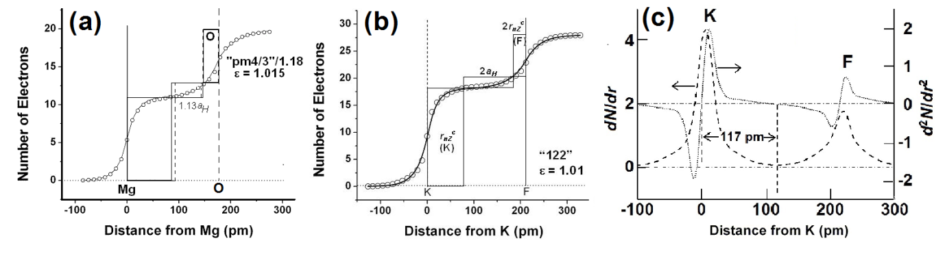
Bond order refs 88, 89
We have found support from B3LYP DFT calculations for the “hub” and “axle” model of eqns 5 and 6.
We use a semi-empirical form of eeff in eqn 11 with
eeff = [1 + a/VX-] = [1 + {ra’/CR–(X)}3] (12)
withVX- = (4p/3)(CR–X)3 and the dielectric polarizability, a = (4p/3)r’a3 using our earlier results21 on polarizability of atoms. The use of eeff in eqn 11 emphasizes the role of polarizability and the volume and points to the importance of environment-dependence. A core size, rexpt(M) is calculated from experimentally observed45,46 inter-atomic distance of various elements at NTP using eqns 11 and 12 (M = X) and using CM = 2.144 and CX = 2.300, while nv (indicated in important cases by superscripts) is obtained32,47 from the nominal position of the atom in the periodic table for calculating FS. The values of rexptagree well (Fig 3) with tabulated values of rnZc of most elements including rare-earth elements and some actinides Ac1, Th2, Cm2, Bk2, Cf2, Es2 and Fm2. Considering the range of atomic number varied (from Z = 1 – 103).
dMXcalc((col(rnZc)*52.9*2.144 – 35.2 + (col(rnZc)*52.9*2.3 +105.6))/(1+0.202*((col(Nv)/2)*(col(Nv)/2+1))^0.333))
We have fitted ~240M-X distances (~ 60 gas-phase diatomic molecules between atoms of insulating elements (Table 1), ~ 90 gas-phase diatomic molecules with at least one atom being that of a metallic element at NTP (Table 2), and ~ 90 solids with rock-salt structure, Table 3) using eMX= 1 (see supporting data and appendix for values of CM. CX and DMX = DM + DX). The best fit (Fig 1) of observed distance, dMX(obs), with the calculated distance dMXCCD, using “charge-transfer” or “neutral” values for CP and DPgives dMX(obs) = 1.03(0.003)dMXCCD. From this fit one may surmise that the average value of eMX = 1.03, which seems to be reasonable. The larger scatter in the case of the solids may be attributed to constraints imposed by X—X and M—M contacts. Except F2 and I2 all other may be fitted using “charge-transfer” (CT) “axle” sizes. All the solids and ~ 50% of the gas-phase compounds require CT “hub sizes”.
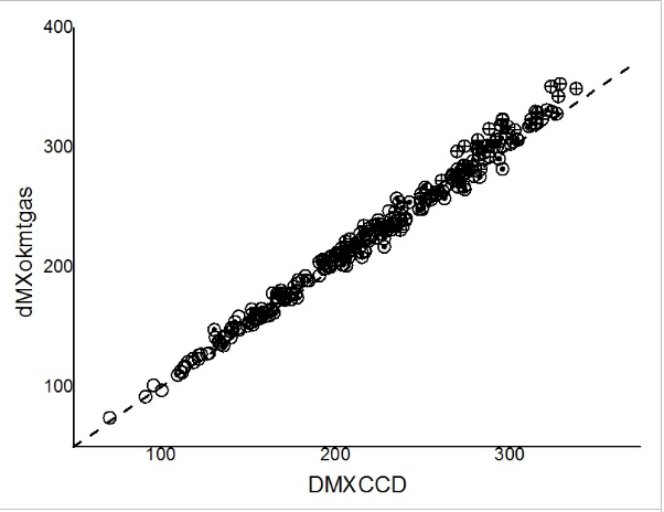
The intermolecular non-bonded distances between atoms is usually thought to be given by the sum of van der Waals’ radii. These radii for atoms have been tabulated by Bondi who refined the earlier work by Pauling. The Bondi radii are “… intrinsically approximate because atoms in molecules are not spherical, whereas assigning them a single radius implies a spherical model.” They are, however, widely used and find empirical validity even if their theoretical modeling has considerable uncertainty. Mantina et al have provided a set of what they call consistent radii for various main-group atoms. We have shown in Fig 2 the plots of these tabulated radii vs rnZc for various atoms. They have been compared with calculated values of CR0vdW, CR0–, 0.5d222 and 0.5(CR0vdW + 0.5dMM00±), which would correspond, respectively, to the van der Waals size, ionic size, half the (nv = 0) “neutral” distance CMCXDMX = 222,and the average of van der Waals size and half the CT bond size, d00±. It is seen from Fig 2 that the tabulated radii is not greater than CRvdW; the van der Waals size for rare-gas atoms in crystals is close to CRvdW;other atoms of insulating elements have radii between CR– and CRvdW; the radii of atoms of metallic elements behave differently.

Fig 2. Plot of tabulated van der Waals’ radii of elements from refs (Bondi, A. J. Phys. Chem. 1964, 68, 441, M. Mantina, A. C. Chamberlin, R. Valero, C. J. Cramer, and D. G. Truhlar, Consistent van der Waals Radii for the Whole Main Group, J. Phys. Chem. A 2009, 113, 5806). The lines show the values expected from eqn 1 and Table 1 for CR0vdW, CR0–, 0.5d222 and the average of CRvdw and 0.5dMM00± (= CR0+ + CR0–).
(¶E/¶r (r))ù) (¶E/¶r(r))r(eq) + (¶E/¶r)r(eq)/(¶r(r)/¶r)ù (12)
The electronegativity equalization principle
states that, in its ground state, the electronegativity of every
component in a system is the same. A paradox then arises:
molecular fragments that are very far apartmust still have the
same electronegativity, which seems to contradict the common
assumption that spatially separated molecular species
can be described independentlyThe electronegativity of atoms and molecules, then, is subject
to a locality paradox2. the electronegativity of the atom
is given by a common value characteristic of the system even
if all the other components of the system are infinitely far
away.
The imposing variety of published theoretical methods for
partitioning a molecular density into AIM contributions, e.g.
refs. 1–15, testifies to the importance of this theme for chemistry.
The different methods are based on different principles, some to
a degree arbitrary (5) or heuristic (15), which can produce
conflicting trends in the associated atomic net charges (effective
oxidation states). Methods differ in the theoretical technique
used, e.g., topological analysis of the density, wave-function
description, or density-functional description. They also differ in
the physicalyheuristic principles invoked, e.g., electronegativity
equalization, zero flux, and minimum-promotion energy rules.
They can have specific disadvantages, e.g., basis set dependence.
The well-known and appealing quantum-topological approach
(1–4) suffers from the fact that its defined atomic densities are
not ‘‘y-representable.’’ [An atomic density is y-representable
when there exists an external potential that has this density as a
ground-state density.]
Transferability is a fundamental concept in the
theory of Atoms in Molecules,45 that is, atoms or
functional groups with similar properties should
have similar electron densities.63 Therefore, the definition
of a similarity measure between atoms or
functional groups provides a means for assessing
quantitatively the degree of transferability of those
atoms or functional groups in molecules. …. the degree of transferability of any two atoms
can be assessed in a quantitative way by calculating
a similarity measure between the corresponding
charge distributions.64
In the recent descriptions11 of ‘fuzzy atoms’ there may be diffusions between one atomic region to another. The concept of ‘fuzzy atoms’ could overcome some of the main drawbacks associated with the use of afixed set of covalent atomic radii for different chemical environments when there is difficulty in accounting for, say, different partial ionic characteris that the same atoms aretreated on equal footing in different chemical environments,i.e., partial ionic character of atoms cannot be properly accountedfor.
In the real space structure of atoms and molecules a fundamental quantity such as the Bohr radius also involves h. There is however the moot point
There is a bridging approach, computed by quantum physics not only the strength of inter-atomic interactions Once the total electron density is known, it can be
analysed in detail by means of its topological properties within
the quantum theory of atoms in molecules (Bader, 1990, 1994).
With such an analysis, one can go beyond a purely qualitative
description of the nature and strength of inter-atomic interactions.
It can also be used to de®ne inter-atomic surfaces
inside which atomic charges and moments are integrated.
BB distance in diborane is 176 pm
In contrast to the common multiple bonding between carbon atoms, multiply bonded boron compounds have still been a synthetic challenge due to the electron deficiency of boron. We now report that a stable doubly hydrogen-bridged diborane(4), EindB(mu-H)(2)BEind, is produced by the two-electron oxidation of a hydrogen-substituted diborane(4) dianion [Li(+)(thf)](2)[Eind(H)BB(H)Eind](2-), where Eind denotes the 1,1,3,3,5,5,7,7-octaethyl-s-hydrindacen-4-yl. The X-ray crystallography reveals a short B-B distance of 1.4879(7) A in comparison with the normal B-B single bond length (1.72 A), the presence of two hydrogen atoms bridged perpendicular to the B-B bond with a butterfly shape having a dihedral angle of the two BHB triangles of 113(1) degrees, and a linear geometry around the B-B bond with a C-B-B bond angle of 178.92(4) degrees. These structural data, experimental electron density analysis, and computational studies confirm the 3-fold bonding (a sigma and two pi-like bonds) between the two boron atoms incorporating the two bridging hydrogen atoms.
It is the purpose of this paper to reach a consensus regarding
the dichotomous approaches to chemistry: one espoused by those
who consider the fundamental concepts of chemistry to lie
beyond the bounds of physics, the other, that chemical observations
and hence the conceptual framework of chemistry are fully
described, predicted, and accounted for by quantum mechanics,
the physics governing the behavior of electrons and nuclei. The
former approach is summarized by Professor Roald Hoffmann
in correspondence with the author dated December, 2007: “I
also have philosophical reservations about the reductionist
framework in which AIM (atoms in molecules) resides; I believe
the most interesting ideas of chemistry are not reducible to
physics. I think we have a fundamental difference of opinion
between us on this matter.”
The conviction exists in the
literature that a proper understanding of the chemical bond is
only possible by looking at delocalization effects which stem
from consideration of the uncertainty principle
<CRS±> = 0.889(5.077) + 0.876(0.033)rSlater(rPearson = 0.95, R = 0.90)
49, 51, 181, 182, 185,196, 197, 198, 199, 201, 202, 203, 205, 224, 225, 227, 230, 231, 233, 234, 237, 239, 241, 249, 245, 146, 248, 249, 250
253, 261, 263
GeSe11, GeIITe, AgIBr, AgICl, AgII, CsBr, CsCl, CsF, CsI, CuIBr, CuICl. CuIF, CuII, KBr,
KCl, KI, LiCl, LiF, LiI, LiLi. MnIH, NaBr. NaF,
AgBr. AgCl, AgF, KH, LiI, MgS, MgSe, NaI, CsH, NaH, RbH, SnSb, SnSe. SnTe, SnAs, PbS, PbSe, PbTe
Appendix
176.15, 140.47, 149 pm. For stoichiometric LiB, the B-B distance in the experimental
structure is 1.40 A˚ . If one electron is transferred from
Li to B, the B− chain is then isoelectronic to C. A carbon
allotrope of such chains has been persistently claimed in the
literature, often called karbin or carbyne.38–40 The structure
of an infinite Cn chain might be a cumulene (all C-C double
bonds) or have alternating single and triple bonds. Either way,
the average C-C distance (therefore the average B-B distance
in an isoelectronic poly-B−) should be short. Can we estimate
how short? A B-B triple bond in a molecule is around 1.56 ˚A41
and a B-B single bond around 1.70 A˚ .
he predicted C2cb-40 to
Cmca-24 transition pressure is 91.3 GPa The semiconducting character of the C2cb-40 structure
can be rationalized from a topological analysis of both the
electron localization function (ELF) and electron density.
The structure is shown in projection down the a axis in
Fig. 4, and can be described in terms of six modulated
layers (ABCA0B0C0) lying perpendicular to the b axis,
where the atomic positions in the primed and unprimed
layers are related by the C-centering translation. BðB0Þ
layers contain the Li2 atoms, while the AðA0Þ and
CðC0Þ layers contain a mix of the other Li atoms.
At 85 GPa, the shortest in-layer Li-Li distance is 1.604A °
compared with 1.783 A ° for the interlayer distance.
114/3 182.5
rnZc(Li3* (1s,2s)3 = 0.33 a.u. rnZc (Li2*(1s, 2sp2)) = 0.50 a.u.
Li3*Li3* pm4/3 = 148 pm, Li3*Li3* 114/3 = 105.4 Li3*Li3* 112 = 140.5, Li3*Li3* 222 = 176.2 Li3*Li3* 212 = 158.7 LiLi 114/3 = 182.5 Li2*Li2*pm4/3 = 188 Li2*Li2* 224/3 = 177 pm LiLi3* 114/3 144pm LiLi3* 112 = 179.2
B-B 214/3 = 141 pm BB pm4/3 = 176.2 BB p1m14/3 = 148/8 BB p2m24/3 = 140.51
The semiconducting character of the C2cb-40 structure
can be rationalized from a topological analysis of both the
electron localization function (ELF) and electron density.
The structure is shown in projection down the a axis in
Fig. 4, and can be described in terms of six modulated
layers (ABCA0B0C0) lying perpendicular to the b axis,
where the atomic positions in the primed and unprimed
layers are related by the C-centering translation. BðB0Þ
layers contain the Li2 atoms, while the AðA0Þ and
CðC0Þ layers contain a mix of the other Li atoms.
At 85 GPa, the shortest in-layer Li-Li distance is 1.604A °
compared with 1.783 A ° for the interlayer distance.
At 85 GPa, the shortest in-layer Li-Li distance is 1.604A °
compared with 1.783 A ° for the interlayer distance (ref 174) The ELF analysis suggests that Li becomes non-metallic at high pressure by localization of the electrons in interstitial regions. ….All of these phases are characterized by the valence electrons occupying interstitial regions, which may become disjoint leading to semiconducting electride phases. This invites further investigation of the role of interstitial electron density in these systems … A peculiarity of the observed oC88 phase at very low temperature is the reported huge increase of resistivity at 25 K (4 orders of magnitude) across its narrow range of stability, interpreted as a phase mixture [8]; no such mixture
is observed in our experiment, albeit at higher temperatures,
and we cannot exclude the possible instability of
oC88to a soft-phonon transition at very low temperatures.
In summary, we have shown that oC88 is metallic with a
large, complex structure with probable C2mb symmetry;
oC40has a C2cb-40 structure not observed previously,
which is nonmetallic with a larger band gap than any
previously found or proposed for Li at any pressure; and
theoC24 phase has the Cmca-24 structure proposed by
Rousseau et al. [6].
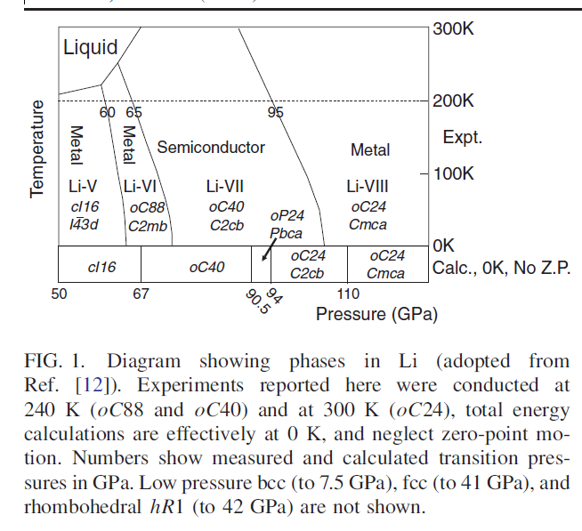
Ref 12 is ref 173
For stoichiometric LiB, the B-B distance in the experimental
structure is 1.40 A˚ .
From ref 177 Liu et al.178obtained the best re®nement of x-ray data for
the hexagonal space group No. 194 (P63 /mmc) with lattice
constantsa54.022 ., c52.796 ..14 In the unit cell with
two formula units ~f.u.!, B and Li occupy the Wyckoff positions
2b ~0,0,1/4! and 2c ~1/3,2/3,1/4!, respectively. The
structure is shown in the top panel of Fig. 1, and consists of
hexagonal sheets of B, with Li lying at interstitial sites
within the B layers in alternating positions along the c axis.
The structure can also be considered from the viewpoint of a
hexagonal array of B chains oriented along the c axis, and
this viewpoint will become more useful below. We will refer
to this structure as a-LiB, from which we begin our investigation
of structures. ………Though WöÈrle and Nesper179suggested the possibility of alternating
single and triple bonds ~1.78 . and 1.40 .! rather
than uniform double bonds ~1.59 .!, their analysis could not
distinguish them. The calculated Fermi surfaces are not suf-
®ciently one dimensional to induce a Peierls distortion. Our
calculated B-B bond length of 1.55 . and the stability
against dimerization strongly favor the latter picture.
a-LiB~experiment! P63 /mmc a=4.022, c=2.796 Li-B = 232 pm
from ref 176 …The lithium-lithium distances 2.13056(9)Å among the zig-zag chains
are comparable to the Li-Li distance reported for Li2B6 [5]. The intra-polyhedral
B-B bond lengths vary from 1.6702(6)Å to 1.8038(3)Å. The inter-polyhedral bond
lengths vary from 1.53472(6)Å to 1.8026(8)Å. The shortest bond length 1.53472(6)Å
can be compared to the average boron-boron distances in LiBx (0.82_ x _ 1) [6] and
the longest boron-boron bond distance 1.8038(3)Å can be compared to that found
for Na3B20 [22].
Our study suggests that the large SO interaction would suppress the Peierls instability which is generally expected to occur in one-dimensional conductors.
The optimized Li-oC8 structure has one short inter-atomic
distance of 1.47 AÊ and four more short contacts at 1.69 to 1.79 AÊ.158
Schematic representation of the cubic crystal structure of Li near 45 GPa. The
space group is I-43d. The cubic cell contains 16 atoms occupying the Wyckoff 16c site
(positional parameter x . 0:055). The shortest inter-atomic distances (2.1AÊ ) are
indicated by thick lines (from ref 158)
Selenium
(Se) and Tellurium (Te), which are isoelectronic elements
to Po in the chalcogen group, also have the trigonal spiral
structure [3]. Note that the trigonal structure can be
derived from the sc structure by elongation or contraction
along the [111] direction [4], which is known to occur due
to the Peierls distortion in p-bonded systems of Se and
Te [5].
Recently, there have been several reports to explore the
origin of the stabilized sc structure in Po [6–11]. General
consensus so far is that the large relativistic effects in Po
play an important role. The Peierls instability tends to
be suppressed in Po by the relativistic effects. However,
there was controversy on the role of spin-orbit coupling
(SOC) of 6p electrons
The simple view that lithium should remain simple under
pressure was challenged by the theoretical prediction that
under compression it would yield lower-coordinated structures
starting at _45GPa, with the orthorombic Cmca
structure being favored above _100GPa (about four fold
compression)2,3. This latter structure can be obtained
continuously from the fcc arrangement to yield a configuration
in which lithium ions are clearly seen to form pairs;
the associated band structure is semimetallic, almost that
of a zero-gap semi-conductor. It was also reported, counter
intuitively, that the valence band width narrowed under
pressure and that the band gaps at the zone faces became
very large compared to the band width, indicating
astrong electron-ion effective interaction, quite at odds
with the original assumption that the alkalis are nearly
free electron metals170.
The essence of this reasoning
resides in an argument that the contact of bands with Brillouin
zone_BZ_ planes, associated with crystal _pseudo_potentials
VK _generally local_, and states near the Fermi level
can be a key stabilizing factor. The value of VK varies in
a_Electronic mail: rh34@cornell.edu. general in complex fashion with density, but straightforward
Although not unheralded (similar
band width narrowing had been reported before in
lithium [2,3,5], but only for the fcc structure, and at a
pressure that would prove well beyond the stability range
of that phase), these calculations offered deep insights into
the origin of the breakdown of nearly free electron behavior.
Indeed, it was argued that the combined effects of
the Pauli exclusion principle and orthogonality render the
ionic cores repulsive to valence states; as the volume of
the sample decreases under pressure, the relative volume
of the rather incompressible cores increases, forcing the
valence density to localize into interstitial regions. As will
be discussed below, this turns out to be a common factor
in the various phases of lithium at high pressure, and can
in fact be taken as a better paradigm than the nearly free
electron approximation [4,6].
.
At least a two-atom property, such as dMX, is required to recognize screening effects since a charge appears screened only to another particle in the same medium.
Transferable core atomic sizes, rnZc, for all elements have been obtained8 from most rudimentary vacuum-polarization ideas from a classical stationary point. These sizes are thus consistent17 with a m = 0 value of the chemical potential18,19 to obtain equilibrium bond distances.
For main group elements, the plot (Fig 1) of <rnZc>vs {rnZc}* indicates that a size lDmet = aH/2 separates insulating elements from metallic ones. Since <rnZc> and {rnZc}* are for excited state properties, the criterion for lDmet is consistent with the view13 that the electrical conductivity is a measure of the probability of coherent or resonant excitation energy transfer. The metallic elements accordingly have resistivity £rmax(FL) » 88 mohm cm, the maximum resistivity13 for Fermi liquids (inset, Fig 1). The metalloid element, As, (lDmet><rnZc>(As) = 0.41 a,u.) has ra< 170 pm but has15,16r<rmax(FL) (see inset of Fig 1)
Because of the inevitability of a perceived many-atom requirement to account for metallic behaviour, there has been little emphasis on finding a relation between any size that is characteristic of a screening length and provides a single-atom metallic criterion for obtaining a charged or neutral description of atoms in the context of bonding. It is nevertheless relevant to ask whether there is an appropriate fundamental atomic size that determines the metallicity of an element. It is then possible to examine the way this fundamental size sets limiting values for the polarizability, electronegativity, bond descriptions involving metallic and insulating elements. We may also discuss how such a distinction between charge-separated and neutral descriptions of chemical bonds follows naturally in accounting for M-X distances in gas-phase diatomic MX compounds (X is an atom of an insulating element), when M is an atom of an insulating or metallic element, respectively. Recently it has been noted that the description of M-X distance, dMX, ingas-phase or isolated diatomic MX compounds (X is an atom of an insulating element) require “charge-transfer” or “neutral” descriptions, respectively, when M is an atom of an insulating or a metallic element, respectively [49, 50]. This is just the situation for exploring the role of a screening length as we discuss below